快速入门教程
先决条件
在阅读本教程之前,你应该知道一点Python。如果你想回顾一下,请参阅Python教程。
如果你希望在本教程中使用示例,你还必须在计算机上安装一些软件。有关说明,请参阅http://scipy.org/install.html。
基础
NumPy的主要对象是同质多维数组。它是一张表,所有元素(通常是数字)的类型都相同,并通过正整数元组索引。在NumPy中,维度称为轴。轴的数目为秩rank。
例如,3D空间中的点的坐标[1, 2, 1]是rank为1的数组,因为它具有一个轴。该轴的长度为3。在下图所示的示例中,数组的rank为2(它是2维的)。第一维度(轴)的长度为2,第二维度的长度为3。
[[ 1., 0., 0.],
 [ 0., 1., 2.]]
NumPy的数组的类称为ndarray。别名为array。请注意,numpy.array与标准Python库的类array.array不同,后者仅处理一维数组并提供较少的功能。ndarray对象的更重要的属性是:
- ndarray.ndim
- 数组的轴(维度)的个数。在Python世界中,维度的数量被称为rank。
- ndarray.shape
- 数组的维度。这是一个整数的元组,表示每个维度中数组的大小。对于具有n行和m列的矩阵,
shape将是(n,m)。因此,shape元组的长度就是rank或维度的个数ndim。 - ndarray.size
- 数组元素的总数。这等于
shape的元素的乘积。 - ndarray.dtype
- 描述数组中元素类型的对象。可以使用标准Python类型创建或指定dtype。另外NumPy提供了自己的类型。例如numpy.int32、numpy.int16和numpy.float64。
- ndarray.itemsize
- 数组中每个元素的字节大小。例如,元素为
float64类型的数组的itemsize为8(=64/8),而complex32类型的数组的comitemsize为4(=32/8)。它等于ndarray.dtype.itemsize。 - ndarray.data
- 该缓冲区包含数组的实际元素。通常,我们不需要使用此属性,因为我们将使用索引访问数组中的元素。
示例
>>> import numpy as np
>>> a = np.arange(15).reshape(3, 5)
>>> a
array([[ 0,  1,  2,  3,  4],
       [ 5,  6,  7,  8,  9],
       [10, 11, 12, 13, 14]])
>>> a.shape
(3, 5)
>>> a.ndim
2
>>> a.dtype.name
'int64'
>>> a.itemsize
8
>>> a.size
15
>>> type(a)
<type 'numpy.ndarray'>
>>> b = np.array([6, 7, 8])
>>> b
array([6, 7, 8])
>>> type(b)
<type 'numpy.ndarray'>
数组创建
有几种方法来创建数组。
例如,你可以使用array函数从常规Python列表或元组中创建数组。得到的数组的类型从序列中元素的类型推导出。
>>> import numpy as np
>>> a = np.array([2,3,4])
>>> a
array([2, 3, 4])
>>> a.dtype
dtype('int64')
>>> b = np.array([1.2, 3.5, 5.1])
>>> b.dtype
dtype('float64')
常见的错误在于用多个数字参数调用array,而不是提供单个数字列表作为参数。
>>> a = np.array(1,2,3,4)    # WRONG
>>> a = np.array([1,2,3,4])  # RIGHT
array将序列的序列转换成二维阵列,将序列的序列的序列转换成三维数组,等等。
>>> b = np.array([(1.5,2,3), (4,5,6)])
>>> b
array([[ 1.5,  2. ,  3. ],
       [ 4. ,  5. ,  6. ]])
数组的类型也可以在创建时明确指定:
>>> c = np.array( [ [1,2], [3,4] ], dtype=complex )
>>> c
array([[ 1.+0.j,  2.+0.j],
       [ 3.+0.j,  4.+0.j]])
通常,数组的元素最初是未知的,但其大小是已知的。因此,NumPy提供了几个函数来创建具有初始占位符内容的数组。这些最小化数组增长的必要,数组增长是一种昂贵的操作。
函数zeros创建一个由0组成的数组,函数ones创建一个由1数组的数组,函数empty内容是随机的并且取决于存储器的状态。默认情况下,创建的数组的dtype为float64。
>>> np.zeros( (3,4) )
array([[ 0.,  0.,  0.,  0.],
       [ 0.,  0.,  0.,  0.],
       [ 0.,  0.,  0.,  0.]])
>>> np.ones( (2,3,4), dtype=np.int16 )                # dtype can also be specified
array([[[ 1, 1, 1, 1],
        [ 1, 1, 1, 1],
        [ 1, 1, 1, 1]],
       [[ 1, 1, 1, 1],
        [ 1, 1, 1, 1],
        [ 1, 1, 1, 1]]], dtype=int16)
>>> np.empty( (2,3) )                                 # uninitialized, output may vary
array([[  3.73603959e-262,   6.02658058e-154,   6.55490914e-260],
       [  5.30498948e-313,   3.14673309e-307,   1.00000000e+000]])
为了创建数字序列,NumPy提供类似于range的函数,返回数组而不是列表。
>>> np.arange( 10, 30, 5 )
array([10, 15, 20, 25])
>>> np.arange( 0, 2, 0.3 )                 # it accepts float arguments
array([ 0. ,  0.3,  0.6,  0.9,  1.2,  1.5,  1.8])
当arange与浮点参数一起使用时,由于浮点数的精度是有限的,通常不可能预测获得的元素数量。出于这个原因,通常最好使用函数linspace,它接收我们想要的元素数量而不是步长作为参数:
>>> from numpy import pi
>>> np.linspace( 0, 2, 9 )                 # 9 numbers from 0 to 2
array([ 0.  ,  0.25,  0.5 ,  0.75,  1.  ,  1.25,  1.5 ,  1.75,  2.  ])
>>> x = np.linspace( 0, 2*pi, 100 )        # useful to evaluate function at lots of points
>>> f = np.sin(x)
打印数组
当打印数组时,NumPy以类似于嵌套列表的方式显示它,但是使用以下布局:
- 最后一个轴从左到右打印,
- 第二个到最后一个从上到下打印,
- 其余的也从上到下打印,每个切片与下一个用空行分开。
一维数组被打印为行、二维为矩阵和三维为矩阵列表。
>>> a = np.arange(6)                         # 1d array
>>> print(a)
[0 1 2 3 4 5]
>>>
>>> b = np.arange(12).reshape(4,3)           # 2d array
>>> print(b)
[[ 0  1  2]
 [ 3  4  5]
 [ 6  7  8]
 [ 9 10 11]]
>>>
>>> c = np.arange(24).reshape(2,3,4)         # 3d array
>>> print(c)
[[[ 0  1  2  3]
  [ 4  5  6  7]
  [ 8  9 10 11]]
 [[12 13 14 15]
  [16 17 18 19]
  [20 21 22 23]]]
有关reshape的详情,请参阅下文。
如果数组太大而无法打印,NumPy会自动跳过数组的中心部分,并只打印边角:
>>> print(np.arange(10000))
[   0    1    2 ..., 9997 9998 9999]
>>>
>>> print(np.arange(10000).reshape(100,100))
[[   0    1    2 ...,   97   98   99]
 [ 100  101  102 ...,  197  198  199]
 [ 200  201  202 ...,  297  298  299]
 ...,
 [9700 9701 9702 ..., 9797 9798 9799]
 [9800 9801 9802 ..., 9897 9898 9899]
 [9900 9901 9902 ..., 9997 9998 9999]]
要禁用此行为并强制NumPy打印整个数组,你可以使用set_printoptions更改打印选项。
>>> np.set_printoptions(threshold='nan')
基本操作
数组上的算术运算符使用元素级别。将创建一个新数组并用结果填充。
>>> a = np.array( [20,30,40,50] )
>>> b = np.arange( 4 )
>>> b
array([0, 1, 2, 3])
>>> c = a-b
>>> c
array([20, 29, 38, 47])
>>> b**2
array([0, 1, 4, 9])
>>> 10*np.sin(a)
array([ 9.12945251, -9.88031624,  7.4511316 , -2.62374854])
>>> a<35
array([ True, True, False, False], dtype=bool)
与许多矩阵语言不同,乘法运算符*的运算在NumPy数组中是元素级别的。可以使用dot函数或方法执行矩阵乘积:
>>> A = np.array( [[1,1],
...             [0,1]] )
>>> B = np.array( [[2,0],
...             [3,4]] )
>>> A*B                         # elementwise product
array([[2, 0],
       [0, 4]])
>>> A.dot(B)                    # matrix product
array([[5, 4],
       [3, 4]])
>>> np.dot(A, B)                # another matrix product
array([[5, 4],
       [3, 4]])
某些操作(如+=和*=)可以修改现有数组,而不是创建新数组。
>>> a = np.ones((2,3), dtype=int)
>>> b = np.random.random((2,3))
>>> a *= 3
>>> a
array([[3, 3, 3],
       [3, 3, 3]])
>>> b += a
>>> b
array([[ 3.417022  ,  3.72032449,  3.00011437],
       [ 3.30233257,  3.14675589,  3.09233859]])
>>> a += b                  # b is not automatically converted to integer type
Traceback (most recent call last):
  ...
TypeError: Cannot cast ufunc add output from dtype('float64') to dtype('int64') with casting rule 'same_kind'
当使用不同类型的数组操作时,结果数组的类型对应于更一般或更精确的数组(称为向上转换的行为)。
>>> a = np.ones(3, dtype=np.int32)
>>> b = np.linspace(0,pi,3)
>>> b.dtype.name
'float64'
>>> c = a+b
>>> c
array([ 1.        ,  2.57079633,  4.14159265])
>>> c.dtype.name
'float64'
>>> d = np.exp(c*1j)
>>> d
array([ 0.54030231+0.84147098j, -0.84147098+0.54030231j,
       -0.54030231-0.84147098j])
>>> d.dtype.name
'complex128'
许多一元操作,例如计算数组中所有元素的和,被实现为ndarray类的方法。
>>> a = np.random.random((2,3))
>>> a
array([[ 0.18626021,  0.34556073,  0.39676747],
       [ 0.53881673,  0.41919451,  0.6852195 ]])
>>> a.sum()
2.5718191614547998
>>> a.min()
0.1862602113776709
>>> a.max()
0.6852195003967595
默认情况下,这些操作适用于数组,就像它是一个数字列表,而不管其形状。但是,通过指定axis参数,你可以沿着数组的指定轴应用操作:
>>> b = np.arange(12).reshape(3,4)
>>> b
array([[ 0,  1,  2,  3],
       [ 4,  5,  6,  7],
       [ 8,  9, 10, 11]])
>>>
>>> b.sum(axis=0)                            # sum of each column
array([12, 15, 18, 21])
>>>
>>> b.min(axis=1)                            # min of each row
array([0, 4, 8])
>>>
>>> b.cumsum(axis=1)                         # cumulative sum along each row
array([[ 0,  1,  3,  6],
       [ 4,  9, 15, 22],
       [ 8, 17, 27, 38]])
通用函数
NumPy提供了熟悉的数学函数,如sin,cos和exp。在NumPy中,这些被称为“通用函数”(ufunc)。在NumPy中,这些函数在数组上按元素级别操作,产生一个数组作为输出。
>>> B = np.arange(3)
>>> B
array([0, 1, 2])
>>> np.exp(B)
array([ 1.        ,  2.71828183,  7.3890561 ])
>>> np.sqrt(B)
array([ 0.        ,  1.        ,  1.41421356])
>>> C = np.array([2., -1., 4.])
>>> np.add(B, C)
array([ 2.,  0.,  6.])
另见
all, any, apply_along_axis, argmax, argmin, argsort, average, bincount, ceil, clip, conj, corrcoef, cov, cross, cumprod, cumsum, diff, dot, floor, inner, inv, lexsort, max, maximum, mean, median, min, minimum, nonzero, outer, prod, re, round, sort, std, sum, trace, transpose, var, vdot, vectorize, where
索引、切片和迭代
一维数组可以索引,切片和迭代,非常类似于列表和其他Python序列。
>>> a = np.arange(10)**3
>>> a
array([  0,   1,   8,  27,  64, 125, 216, 343, 512, 729])
>>> a[2]
8
>>> a[2:5]
array([ 8, 27, 64])
>>> a[:6:2] = -1000    # equivalent to a[0:6:2] = -1000; from start to position 6, exclusive, set every 2nd element to -1000
>>> a
array([-1000,     1, -1000,    27, -1000,   125,   216,   343,   512,   729])
>>> a[ : :-1]                                 # reversed a
array([  729,   512,   343,   216,   125, -1000,    27, -1000,     1, -1000])
>>> for i in a:
...     print(i**(1/3.))
...
nan
1.0
nan
3.0
nan
5.0
6.0
7.0
8.0
9.0
多维数组每个轴可以有一个索引。这些索引以逗号分隔的元组给出:
>>> def f(x,y):
...     return 10*x+y
...
>>> b = np.fromfunction(f,(5,4),dtype=int)
>>> b
array([[ 0,  1,  2,  3],
       [10, 11, 12, 13],
       [20, 21, 22, 23],
       [30, 31, 32, 33],
       [40, 41, 42, 43]])
>>> b[2,3]
23
>>> b[0:5, 1]                       # each row in the second column of b
array([ 1, 11, 21, 31, 41])
>>> b[ : ,1]                        # equivalent to the previous example
array([ 1, 11, 21, 31, 41])
>>> b[1:3, : ]                      # each column in the second and third row of b
array([[10, 11, 12, 13],
       [20, 21, 22, 23]])
当提供比轴数更少的索引时,缺失的索引被认为是一个完整切片:
>>> b[-1]                                  # the last row. Equivalent to b[-1,:]
array([40, 41, 42, 43])
b[i]方括号中的表达式i被视为后面紧跟着:的多个实例,用于表示剩余轴。NumPy也允许你使用三个点写为b[i,...]。
三个点(...)表示产生完整索引元组所需的冒号。例如,如果x是rank为的5数组(即,它具有5个轴),则
x[1,2,...]等效于x[1,2,:,:,:]x[...,3]到x[:,:,:,:,3]x[4,...,5,:]到x[4,:,:,5,:]
>>> c = np.array( [[[  0,  1,  2],               # a 3D array (two stacked 2D arrays)
...                 [ 10, 12, 13]],
...                [[100,101,102],
...                 [110,112,113]]])
>>> c.shape
(2, 2, 3)
>>> c[1,...]                                   # same as c[1,:,:] or c[1]
array([[100, 101, 102],
       [110, 112, 113]])
>>> c[...,2]                                   # same as c[:,:,2]
array([[  2,  13],
       [102, 113]])
对多维数组的迭代是相对于第一个轴完成的:
>>> for row in b:
...     print(row)
...
[0 1 2 3]
[10 11 12 13]
[20 21 22 23]
[30 31 32 33]
[40 41 42 43]
但是,如果想对数组中的每个元素执行一个操作,可以使用flat属性,它是一个迭代器
>>> for element in b.flat:
...     print(element)
...
0
1
2
3
10
11
12
13
20
21
22
23
30
31
32
33
40
41
42
43
另见
形状操作
更改数组的形状
数组具有由沿着每个轴的元素数量给出的形状:
>>> a = np.floor(10*np.random.random((3,4)))
>>> a
array([[ 2.,  8.,  0.,  6.],
       [ 4.,  5.,  1.,  1.],
       [ 8.,  9.,  3.,  6.]])
>>> a.shape
(3, 4)
可以使用各种命令更改数组的形状。请注意,以下三个命令都返回修改的数组,但不更改原始数组:
>>> a.ravel()  # returns the array, flattened
array([ 2.,  8.,  0.,  6.,  4.,  5.,  1.,  1.,  8.,  9.,  3.,  6.])
>>> a.reshape(6,2)  # returns the array with a modified shape
array([[ 2.,  8.],
       [ 0.,  6.],
       [ 4.,  5.],
       [ 1.,  1.],
       [ 8.,  9.],
       [ 3.,  6.]])
>>> a.T  # returns the array, transposed
array([[ 2.,  4.,  8.],
       [ 8.,  5.,  9.],
       [ 0.,  1.,  3.],
       [ 6.,  1.,  6.]])
>>> a.T.shape
(4, 3)
>>> a.shape
(3, 4)
由ravel()产生的数组中元素的顺序通常是“C风格”,也就是说,最右边的索引“改变最快”,所以[0,0]之后的元素是[0,1] 。如果数组被重塑成某种其他形状,则该数组也被视为“C风格”。NumPy通常创建按此顺序存储的数组,因此ravel()通常不需要复制其参数,但如果数组是通过对另一个数组进行切片或使用不寻常的选项创建的,则可能需要复制。还可以使用可选参数来指示函数ravel()和reshape(),以使用FORTRAN式数组,其中最左侧的索引改变最快。
reshape函数返回其修改形状的参数,而ndarray.resize方法修改数组本身:
>>> a
array([[ 2.,  8.,  0.,  6.],
       [ 4.,  5.,  1.,  1.],
       [ 8.,  9.,  3.,  6.]])
>>> a.resize((2,6))
>>> a
array([[ 2.,  8.,  0.,  6.,  4.,  5.],
       [ 1.,  1.,  8.,  9.,  3.,  6.]])
如果在reshape操作中将维度指定为-1,则会自动计算其他维度:
>>> a.reshape(3,-1)
array([[ 2.,  8.,  0.,  6.],
       [ 4.,  5.,  1.,  1.],
       [ 8.,  9.,  3.,  6.]])
将不同数组堆叠在一起
几个数组可以沿不同的轴堆叠在一起:
>>> a = np.floor(10*np.random.random((2,2)))
>>> a
array([[ 8.,  8.],
       [ 0.,  0.]])
>>> b = np.floor(10*np.random.random((2,2)))
>>> b
array([[ 1.,  8.],
       [ 0.,  4.]])
>>> np.vstack((a,b))
array([[ 8.,  8.],
       [ 0.,  0.],
       [ 1.,  8.],
       [ 0.,  4.]])
>>> np.hstack((a,b))
array([[ 8.,  8.,  1.,  8.],
       [ 0.,  0.,  0.,  4.]])
函数column_stack将1D数组作为列堆叠到2D数组中。它等同于仅用于2D数组的hstack:
>>> from numpy import newaxis
>>> np.column_stack((a,b))     # with 2D arrays
array([[ 8.,  8.,  1.,  8.],
       [ 0.,  0.,  0.,  4.]])
>>> a = np.array([4.,2.])
>>> b = np.array([3.,8.])
>>> np.column_stack((a,b))     # returns a 2D array
array([[ 4., 3.],
       [ 2., 8.]])
>>> np.hstack((a,b))           # the result is different
array([ 4., 2., 3., 8.])
>>> a[:,newaxis]               # this allows to have a 2D columns vector
array([[ 4.],
       [ 2.]])
>>> np.column_stack((a[:,newaxis],b[:,newaxis]))
array([[ 4.,  3.],
       [ 2.,  8.]])
>>> np.hstack((a[:,newaxis],b[:,newaxis]))   # the result is the same
array([[ 4.,  3.],
       [ 2.,  8.]])
另一方面,对于任何输入数组,函数row_stack等效于vstack。一般来说,对于具有两个以上维度的数组,hstack沿第二轴堆叠,vstack沿第一轴堆叠,concatenate允许一个可选参数,给出串接应该发生的轴。
注意
在复杂情况下,r_和c_可用于通过沿一个轴堆叠数字来创建数组。它们允许使用范围文字(“:”)
>>> np.r_[1:4,0,4]
array([1, 2, 3, 0, 4])
当以数组作为参数使用时,r_和c_类似于其默认行为中的vstack和hstack,但是允许一个可选参数给出要沿其连接的轴的编号。
将一个数组分成几个较小的数组
使用hsplit,可以沿其水平轴拆分数组,通过指定要返回的均匀划分的数组数量,或通过指定要在其后进行划分的列:
>>> a = np.floor(10*np.random.random((2,12)))
>>> a
array([[ 9.,  5.,  6.,  3.,  6.,  8.,  0.,  7.,  9.,  7.,  2.,  7.],
       [ 1.,  4.,  9.,  2.,  2.,  1.,  0.,  6.,  2.,  2.,  4.,  0.]])
>>> np.hsplit(a,3)   # Split a into 3
[array([[ 9.,  5.,  6.,  3.],
       [ 1.,  4.,  9.,  2.]]), array([[ 6.,  8.,  0.,  7.],
       [ 2.,  1.,  0.,  6.]]), array([[ 9.,  7.,  2.,  7.],
       [ 2.,  2.,  4.,  0.]])]
>>> np.hsplit(a,(3,4))   # Split a after the third and the fourth column
[array([[ 9.,  5.,  6.],
       [ 1.,  4.,  9.]]), array([[ 3.],
       [ 2.]]), array([[ 6.,  8.,  0.,  7.,  9.,  7.,  2.,  7.],
       [ 2.,  1.,  0.,  6.,  2.,  2.,  4.,  0.]])]
vsplit沿垂直轴分割,array_split允许指定沿哪个轴分割。
复制和视图
当计算和操作数组时,它们的数据有时被复制到新的数组中,有时不复制。这通常是初学者的混乱的来源。有三种情况:
完全不复制
简单赋值不会创建数组对象或其数据的拷贝。
>>> a = np.arange(12)
>>> b = a            # no new object is created
>>> b is a           # a and b are two names for the same ndarray object
True
>>> b.shape = 3,4    # changes the shape of a
>>> a.shape
(3, 4)
Python将可变对象作为引用传递,因此函数调用不会复制。
>>> def f(x):
...     print(id(x))
...
>>> id(a)                           # id is a unique identifier of an object
148293216
>>> f(a)
148293216
视图或浅复制
不同的数组对象可以共享相同的数据。view方法创建一个新数组对象,该对象看到相同的数据。
>>> c = a.view()
>>> c is a
False
>>> c.base is a                        # c is a view of the data owned by a
True
>>> c.flags.owndata
False
>>>
>>> c.shape = 2,6                      # a's shape doesn't change
>>> a.shape
(3, 4)
>>> c[0,4] = 1234                      # a's data changes
>>> a
array([[   0,    1,    2,    3],
       [1234,    5,    6,    7],
       [   8,    9,   10,   11]])
对数组切片返回一个视图:
>>> s = a[ : , 1:3]     # spaces added for clarity; could also be written "s = a[:,1:3]"
>>> s[:] = 10           # s[:] is a view of s. Note the difference between s=10 and s[:]=10
>>> a
array([[   0,   10,   10,    3],
       [1234,   10,   10,    7],
       [   8,   10,   10,   11]])
深复制
copy方法生成数组及其数据的完整拷贝。
>>> d = a.copy()                          # a new array object with new data is created
>>> d is a
False
>>> d.base is a                           # d doesn't share anything with a
False
>>> d[0,0] = 9999
>>> a
array([[   0,   10,   10,    3],
       [1234,   10,   10,    7],
       [   8,   10,   10,   11]])
函数和方法概述
这里是一些有用的NumPy函数和方法名称按类别排序的列表。有关完整列表,请参见Routines。
- 数组创建
arange,array,copy,empty,empty_like,eye,fromfile,fromfunction,identity,linspace,logspace,mgrid,ogrid,ones,ones_like, r,zeros,zeros_like- 转换
ndarray.astype,atleast_1d,atleast_2d,atleast_3d,mat- 操纵
array_split,column_stack,concatenate,diagonal,dsplit,dstack,hsplit,hstack,ndarray.item,newaxis,ravel,repeat,reshape,resize,squeeze,swapaxes,take,transpose,vsplit,vstack- 问题
all,any,nonzero,where- 顺序
argmax,argmin,argsort,max,min,ptp,searchsorted,sort- 操作
choose,compress,cumprod,cumsum,inner,ndarray.fill,imag,prod,put,putmask,real,sum- 基本统计
cov,mean,std,var- 基本线性代数
cross,dot,outer,linalg.svd,vdot
Less Basic
Broadcasting规则
Broadcasting允许通用函数以有意义的方式处理具有不完全相同形状的输入。
Broadcasting的第一个规则是,如果所有输入数组不具有相同数量的维度,则“1”将被重复地添加到较小数组的形状,直到所有数组具有相同数量的维度。
Broadcasting的第二个规则确保沿着特定维度具有大小为1的数组表现得好像它们具有沿着该维度具有最大形状的数组的大小。假定数组元素的值沿“Broadcasting”数组的该维度相同。
应用广播规则后,所有数组的大小必须匹配。有关详细信息,请参见Broadcasting。
花式索引和索引技巧
NumPy提供了比常规Python序列更多的索引能力。除了通过整数和切片索引之外,如前所述,数组可以由整数数组和布尔数组索引。
使用索引数组索引
>>> a = np.arange(12)**2                       # the first 12 square numbers
>>> i = np.array( [ 1,1,3,8,5 ] )              # an array of indices
>>> a[i]                                       # the elements of a at the positions i
array([ 1,  1,  9, 64, 25])
>>>
>>> j = np.array( [ [ 3, 4], [ 9, 7 ] ] )      # a bidimensional array of indices
>>> a[j]                                       # the same shape as j
array([[ 9, 16],
       [81, 49]])
当被索引的数组a是多维的时候,单个索引数组指的是a的第一个维度。以下示例通过使用调色板将标签的图像转换为彩色图像来显示此行为。
>>> palette = np.array( [ [0,0,0],                # black
...                       [255,0,0],              # red
...                       [0,255,0],              # green
...                       [0,0,255],              # blue
...                       [255,255,255] ] )       # white
>>> image = np.array( [ [ 0, 1, 2, 0 ],           # each value corresponds to a color in the palette
...                     [ 0, 3, 4, 0 ]  ] )
>>> palette[image]                            # the (2,4,3) color image
array([[[  0,   0,   0],
        [255,   0,   0],
        [  0, 255,   0],
        [  0,   0,   0]],
       [[  0,   0,   0],
        [  0,   0, 255],
        [255, 255, 255],
        [  0,   0,   0]]])
我们还可以为多个维度提供索引。每个维度的索引数组必须具有相同的形状。
>>> a = np.arange(12).reshape(3,4)
>>> a
array([[ 0,  1,  2,  3],
       [ 4,  5,  6,  7],
       [ 8,  9, 10, 11]])
>>> i = np.array( [ [0,1],                        # indices for the first dim of a
...                 [1,2] ] )
>>> j = np.array( [ [2,1],                        # indices for the second dim
...                 [3,3] ] )
>>>
>>> a[i,j]                                     # i and j must have equal shape
array([[ 2,  5],
       [ 7, 11]])
>>>
>>> a[i,2]
array([[ 2,  6],
       [ 6, 10]])
>>>
>>> a[:,j]                                     # i.e., a[ : , j]
array([[[ 2,  1],
        [ 3,  3]],
       [[ 6,  5],
        [ 7,  7]],
       [[10,  9],
        [11, 11]]])
当然,我们可以把i和j放在一个序列中(比如一个列表),然后用列表做索引。
>>> l = [i,j]
>>> a[l]                                       # equivalent to a[i,j]
array([[ 2,  5],
       [ 7, 11]])
但是,我们不能将i和j放入一个数组中,因为这个数组将被解释为索引第一个维度。
>>> s = np.array( [i,j] )
>>> a[s]                                       # not what we want
Traceback (most recent call last):
  File "<stdin>", line 1, in ?
IndexError: index (3) out of range (0<=index<=2) in dimension 0
>>>
>>> a[tuple(s)]                                # same as a[i,j]
array([[ 2,  5],
       [ 7, 11]])
另一个常见的使用数组索引的方法是搜索时间相关系列的最大值:
>>> time = np.linspace(20, 145, 5)                 # time scale
>>> data = np.sin(np.arange(20)).reshape(5,4)      # 4 time-dependent series
>>> time
array([  20.  ,   51.25,   82.5 ,  113.75,  145.  ])
>>> data
array([[ 0.        ,  0.84147098,  0.90929743,  0.14112001],
       [-0.7568025 , -0.95892427, -0.2794155 ,  0.6569866 ],
       [ 0.98935825,  0.41211849, -0.54402111, -0.99999021],
       [-0.53657292,  0.42016704,  0.99060736,  0.65028784],
       [-0.28790332, -0.96139749, -0.75098725,  0.14987721]])
>>>
>>> ind = data.argmax(axis=0)                   # index of the maxima for each series
>>> ind
array([2, 0, 3, 1])
>>>
>>> time_max = time[ ind]                       # times corresponding to the maxima
>>>
>>> data_max = data[ind, xrange(data.shape[1])] # => data[ind[0],0], data[ind[1],1]...
>>>
>>> time_max
array([  82.5 ,   20.  ,  113.75,   51.25])
>>> data_max
array([ 0.98935825,  0.84147098,  0.99060736,  0.6569866 ])
>>>
>>> np.all(data_max == data.max(axis=0))
True
你还可以使用数组索引作为目标来赋值:
>>> a = np.arange(5)
>>> a
array([0, 1, 2, 3, 4])
>>> a[[1,3,4]] = 0
>>> a
array([0, 0, 2, 0, 0])
但是,当索引列表包含重复时,赋值完成多次,留下最后一个值:
>>> a = np.arange(5)
>>> a[[0,0,2]]=[1,2,3]
>>> a
array([2, 1, 3, 3, 4])
这是足够合理的,但如果你想使用Python的+=构造要小心,因为它可能不会做你想要的:
>>> a = np.arange(5)
>>> a[[0,0,2]]+=1
>>> a
array([1, 1, 3, 3, 4])
即使0在索引列表中出现两次,第0个元素也只增加一次。这是因为Python要求“a + = 1”等同于“a = a + 1”。
使用布尔数组索引
当我们用(整数)索引数组索引数组时,我们提供要选取的索引列表。使用布尔索引,方法是不同的;我们明确地选择数组中的哪些元素我们想要的,哪些不是。
对于布尔索引,最自然的方法是使用与原始数组具有相同形状的布尔数组:
>>> a = np.arange(12).reshape(3,4)
>>> b = a > 4
>>> b                                          # b is a boolean with a's shape
array([[False, False, False, False],
       [False,  True,  True,  True],
       [ True,  True,  True,  True]], dtype=bool)
>>> a[b]                                       # 1d array with the selected elements
array([ 5,  6,  7,  8,  9, 10, 11])
此属性在赋值时非常有用:
>>> a[b] = 0                                   # All elements of 'a' higher than 4 become 0
>>> a
array([[0, 1, 2, 3],
       [4, 0, 0, 0],
       [0, 0, 0, 0]])
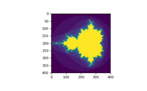
你可以查看以下示例,了解如何使用布尔索引生成Mandelbrot集的图像:
>>> import numpy as np
>>> import matplotlib.pyplot as plt
>>> def mandelbrot( h,w, maxit=20 ):
...     """Returns an image of the Mandelbrot fractal of size (h,w)."""
...     y,x = np.ogrid[ -1.4:1.4:h*1j, -2:0.8:w*1j ]
...     c = x+y*1j
...     z = c
...     divtime = maxit + np.zeros(z.shape, dtype=int)
...
...     for i in range(maxit):
...         z = z**2 + c
...         diverge = z*np.conj(z) > 2**2            # who is diverging
...         div_now = diverge & (divtime==maxit)  # who is diverging now
...         divtime[div_now] = i                  # note when
...         z[diverge] = 2                        # avoid diverging too much
...
...     return divtime
>>> plt.imshow(mandelbrot(400,400))
>>> plt.show()

使用布尔索引的第二种方法更类似于整数索引;对于数组的每个维度,我们给出一个1D布尔数组,选择我们想要的切片:
>>> a = np.arange(12).reshape(3,4)
>>> b1 = np.array([False,True,True])             # first dim selection
>>> b2 = np.array([True,False,True,False])       # second dim selection
>>>
>>> a[b1,:]                                   # selecting rows
array([[ 4,  5,  6,  7],
       [ 8,  9, 10, 11]])
>>>
>>> a[b1]                                     # same thing
array([[ 4,  5,  6,  7],
       [ 8,  9, 10, 11]])
>>>
>>> a[:,b2]                                   # selecting columns
array([[ 0,  2],
       [ 4,  6],
       [ 8, 10]])
>>>
>>> a[b1,b2]                                  # a weird thing to do
array([ 4, 10])
请注意,1D布尔数组的长度必须与你要切片的维度(或轴)的长度一致。在前面的示例中,b1是rank为1的数组,其长度为3(a中行的数量),b2(长度4)适合于索引a的第二个rank(列)。
ix_()函数
ix_函数可以用于组合不同的向量,以便获得每个n-uplet的结果。例如,如果要计算从向量a、b和c中的取得的所有三元组的所有a + b * c:
>>> a = np.array([2,3,4,5])
>>> b = np.array([8,5,4])
>>> c = np.array([5,4,6,8,3])
>>> ax,bx,cx = np.ix_(a,b,c)
>>> ax
array([[[2]],
       [[3]],
       [[4]],
       [[5]]])
>>> bx
array([[[8],
        [5],
        [4]]])
>>> cx
array([[[5, 4, 6, 8, 3]]])
>>> ax.shape, bx.shape, cx.shape
((4, 1, 1), (1, 3, 1), (1, 1, 5))
>>> result = ax+bx*cx
>>> result
array([[[42, 34, 50, 66, 26],
        [27, 22, 32, 42, 17],
        [22, 18, 26, 34, 14]],
       [[43, 35, 51, 67, 27],
        [28, 23, 33, 43, 18],
        [23, 19, 27, 35, 15]],
       [[44, 36, 52, 68, 28],
        [29, 24, 34, 44, 19],
        [24, 20, 28, 36, 16]],
       [[45, 37, 53, 69, 29],
        [30, 25, 35, 45, 20],
        [25, 21, 29, 37, 17]]])
>>> result[3,2,4]
17
>>> a[3]+b[2]*c[4]
17
你还可以如下实现reduce:
>>> def ufunc_reduce(ufct, *vectors):
...    vs = np.ix_(*vectors)
...    r = ufct.identity
...    for v in vs:
...        r = ufct(r,v)
...    return r
然后将其用作:
>>> ufunc_reduce(np.add,a,b,c)
array([[[15, 14, 16, 18, 13],
        [12, 11, 13, 15, 10],
        [11, 10, 12, 14,  9]],
       [[16, 15, 17, 19, 14],
        [13, 12, 14, 16, 11],
        [12, 11, 13, 15, 10]],
       [[17, 16, 18, 20, 15],
        [14, 13, 15, 17, 12],
        [13, 12, 14, 16, 11]],
       [[18, 17, 19, 21, 16],
        [15, 14, 16, 18, 13],
        [14, 13, 15, 17, 12]]])
与正常的ufunc.reduce相比,这个版本的reduce的优点是它使用Broadcasting规则,以避免创建参数数组输出的大小乘以向量的数量。
线性代数
继续工作。这里包括基本线性代数。
简单数组操作
有关更多信息,请参阅numpy目录中的linalg.py。
>>> import numpy as np
>>> a = np.array([[1.0, 2.0], [3.0, 4.0]])
>>> print(a)
[[ 1.  2.]
 [ 3.  4.]]

>>> a.transpose()
array([[ 1.,  3.],
       [ 2.,  4.]])

>>> np.linalg.inv(a)
array([[-2. ,  1. ],
       [ 1.5, -0.5]])

>>> u = np.eye(2) # unit 2x2 matrix; "eye" represents "I"
>>> u
array([[ 1.,  0.],
       [ 0.,  1.]])
>>> j = np.array([[0.0, -1.0], [1.0, 0.0]])

>>> np.dot (j, j) # matrix product
array([[-1.,  0.],
       [ 0., -1.]])

>>> np.trace(u)  # trace
2.0

>>> y = np.array([[5.], [7.]])
>>> np.linalg.solve(a, y)
array([[-3.],
       [ 4.]])

>>> np.linalg.eig(j)
(array([ 0.+1.j,  0.-1.j]), array([[ 0.70710678+0.j        ,  0.70710678-0.j        ],
       [ 0.00000000-0.70710678j,  0.00000000+0.70710678j]]))
Parameters:
    square matrix
Returns
    The eigenvalues, each repeated according to its multiplicity.
    The normalized (unit "length") eigenvectors, such that the
    column ``v[:,i]`` is the eigenvector corresponding to the
    eigenvalue ``w[i]`` .
技巧和提示
这里我们给出一个简短有用的提示。
“自动”Reshape
要更改数组的大小,你可以省略其中一个size,它将被自动推导出来:
>>> a = np.arange(30)
>>> a.shape = 2,-1,3  # -1 means "whatever is needed"
>>> a.shape
(2, 5, 3)
>>> a
array([[[ 0,  1,  2],
        [ 3,  4,  5],
        [ 6,  7,  8],
        [ 9, 10, 11],
        [12, 13, 14]],
       [[15, 16, 17],
        [18, 19, 20],
        [21, 22, 23],
        [24, 25, 26],
        [27, 28, 29]]])
向量堆叠
我们如何从等大小的行向量列表中构造一个二维数组?在MATLAB中这是很容易的:如果x和y是两个相同长度的向量,你只需要m=[x;y] 。在NumPy中,这通过函数column_stack,dstack,hstack和vstack工作,具体取决于要做什么堆叠。例如:
x = np.arange(0,10,2)                     # x=([0,2,4,6,8])
y = np.arange(5)                          # y=([0,1,2,3,4])
m = np.vstack([x,y])                      # m=([[0,2,4,6,8],
                                          #     [0,1,2,3,4]])
xy = np.hstack([x,y])                     # xy =([0,2,4,6,8,0,1,2,3,4])
这些函数背后的逻辑在两个维度可能很奇怪。
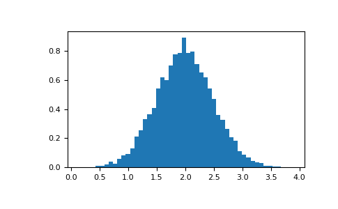
Histograms
NumPy的histogram函数应用于一个数组,并返回一对向量:数组的histogram和向量的bin。注意:matplotlib也具有构建histograms的函数(在Matlab中称为hist),它与NumPy中的不同。主要区别是pylab.hist自动绘制histogram,而numpy.histogram仅生成数据。
>>> import numpy as np
>>> import matplotlib.pyplot as plt
>>> # Build a vector of 10000 normal deviates with variance 0.5^2 and mean 2
>>> mu, sigma = 2, 0.5
>>> v = np.random.normal(mu,sigma,10000)
>>> # Plot a normalized histogram with 50 bins
>>> plt.hist(v, bins=50, normed=1)       # matplotlib version (plot)
>>> plt.show()

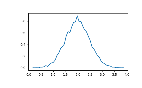
>>> # Compute the histogram with numpy and then plot it
>>> (n, bins) = np.histogram(v, bins=50, normed=True)  # NumPy version (no plot)
>>> plt.plot(.5*(bins[1:]+bins[:-1]), n)
>>> plt.show()
