Hybrid Monte-Carlo Sampling

注意

这是一个高级教程，显示了如何使用Theano实现混合蒙特卡罗（HMC）采样。我们假设读者已经熟悉Theano和基于能量的模型，如RBM。

注意

此部分的代码可从此处下载。

理论

基于能量的模型的最大似然学习需要一个稳健的算法来对负相粒子进行采样（见式(4) of the Restricted Boltzmann Machines (RBM) tutorial). 当使用CD或PCD训练RBM时，通常使用块吉布斯采样来完成，其中条件分布和用作马尔可夫链的转换算子。

然而，在某些情况下，这些条件分布可能难以从（即，需要昂贵的矩阵反转，如在“均值协方差RBM”的情况下）进行采样。此外，即使Gibbs采样可以有效地完成，但是它仍然通过随机游走来进行，这对于某些分布可能不是统计上有效的。在这种情况下，当从连续变量采样时，混合蒙特卡罗（HMC）可以证明是一个强大的工具[Duane87]。它通过模拟由哈密顿动力学控制的物理系统来避免随机行走行为，可能避免过程中的棘手条件分布。

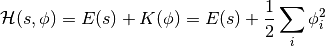
在HMC中，通过模拟物理系统获得模型样本，其中颗粒围绕高维景观移动，受到潜在和动能。使来自[Neal93]的符号适应，粒子通过位置向量或状态和速度向量来表征。颗粒的组合状态表示为。然后将哈密顿量定义为势能（由基于能量的模型定义的相同能量函数）和动能的总和如下：

代替直接采样，HMC通过从规范分布采样来操作。因为两个变量是独立的，边缘化是微不足道的，并且恢复了原始的感兴趣的分布。

哈密顿动力学

修改状态和速度，使得在整个模拟中保持恒定。微分方程由下式给出：

（1）

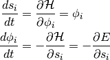
如[Neal93]中所示，上述转换保留了体积并且是可逆的。因此，上述动力学可以用作马尔可夫链的转换算子，并且将保持不变。该链本身不是遍历的，因为模拟动态维持固定的哈密尔顿算子。HMC因此交替汉密尔顿动态步骤，用吉布斯速度采样。因为和是独立的，所以从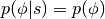开始，采样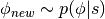是微不足道的，其中通常被认为是单变量高斯。

Leap-Frog算法

在实践中，我们不能模拟哈密顿动力学正是因为时间离散的问题。有几种方法可以做到这一点。为了保持马尔科夫链的不变性，必须注意保持体积守恒和时间可逆性的性质。leap-frog算法维护这些属性并在3个步骤中操作：

（2）

因此，我们在时间执行速度的半步更新，然后用于计算和。

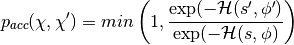
接受/拒绝

在实践中，使用有限步长将不能精确保留并且将在模拟中引入偏差。此外，由于使用浮点数的舍入误差意味着上述变换将不是完全可逆的。

HMC通过在 leapfrog步骤之后添加Metropolis接受/拒绝阶段，在完全取消这些影响。新状态被接受概率，定义为：

HMC算法

在本教程中，我们获得一个新的HMC样本如下：

1. 从单变量高斯分布中采样新速度
2. 请执行 leapfrog步骤以获取新状态
3. 执行接受/拒绝移动

使用Theano实现HMC

在Theano，更新字典和共享变量提供了一种自然的方式来实现抽样算法。采样器的当前状态可以表示为Theano共享变量，其中HMC更新由Theano函数的更新列表实现。

我们将HMC算法分解为以下子分量：

• ：一个符号Python函数，给定初始位置和速度，将执行跳跃更新并返回建议状态的符号变量。
• ：给出起始位置的符号Python函数，通过随机采样速度向量生成。然后它调用并确定是否要接受转换。
• ：一个Python函数，它给出符号输出，生成HMC的单次迭代的更新列表。
• ：一个Python帮助器类，将所有内容封装在一起。

simulate_dynamics

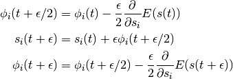
要执行跳跃步骤，我们首先需要定义一个可以迭代的函数。代替实现方程。(2) verbatim, notice that we can obtain and by performing an initial half-step update for , followed by full-step updates for and one last half-step update for . 在循环形式中，这给出：

（3）

上述定义的内循环由以下函数实现，，和分别替换为和。

    def leapfrog(pos, vel, step):
        """
        Inside loop of Scan. Performs one step of leapfrog update, using
        Hamiltonian dynamics.

        Parameters
        ----------
        pos: theano matrix
            in leapfrog update equations, represents pos(t), position at time t
        vel: theano matrix
            in leapfrog update equations, represents vel(t - stepsize/2),
            velocity at time (t - stepsize/2)
        step: theano scalar
            scalar value controlling amount by which to move

        Returns
        -------
        rval1: [theano matrix, theano matrix]
            Symbolic theano matrices for new position pos(t + stepsize), and
            velocity vel(t + stepsize/2)
        rval2: dictionary
            Dictionary of updates for the Scan Op
        """
        # from pos(t) and vel(t-stepsize//2), compute vel(t+stepsize//2)
        dE_dpos = TT.grad(energy_fn(pos).sum(), pos)
        new_vel = vel - step * dE_dpos
        # from vel(t+stepsize//2) compute pos(t+stepsize)
        new_pos = pos + step * new_vel
        return [new_pos, new_vel], {}

函数执行等式的完整算法。（3）。我们从的初始半步更新和的全步开始，然后扫描方法次。

def simulate_dynamics(initial_pos, initial_vel, stepsize, n_steps, energy_fn):
    """
    Return final (position, velocity) obtained after an `n_steps` leapfrog
    updates, using Hamiltonian dynamics.

    Parameters
    ----------
    initial_pos: shared theano matrix
        Initial position at which to start the simulation
    initial_vel: shared theano matrix
        Initial velocity of particles
    stepsize: shared theano scalar
        Scalar value controlling amount by which to move
    energy_fn: python function
        Python function, operating on symbolic theano variables, used to
        compute the potential energy at a given position.

    Returns
    -------
    rval1: theano matrix
        Final positions obtained after simulation
    rval2: theano matrix
        Final velocity obtained after simulation
    """

    def leapfrog(pos, vel, step):
        """
        Inside loop of Scan. Performs one step of leapfrog update, using
        Hamiltonian dynamics.

        Parameters
        ----------
        pos: theano matrix
            in leapfrog update equations, represents pos(t), position at time t
        vel: theano matrix
            in leapfrog update equations, represents vel(t - stepsize/2),
            velocity at time (t - stepsize/2)
        step: theano scalar
            scalar value controlling amount by which to move

        Returns
        -------
        rval1: [theano matrix, theano matrix]
            Symbolic theano matrices for new position pos(t + stepsize), and
            velocity vel(t + stepsize/2)
        rval2: dictionary
            Dictionary of updates for the Scan Op
        """
        # from pos(t) and vel(t-stepsize//2), compute vel(t+stepsize//2)
        dE_dpos = TT.grad(energy_fn(pos).sum(), pos)
        new_vel = vel - step * dE_dpos
        # from vel(t+stepsize//2) compute pos(t+stepsize)
        new_pos = pos + step * new_vel
        return [new_pos, new_vel], {}

    # compute velocity at time-step: t + stepsize//2
    initial_energy = energy_fn(initial_pos)
    dE_dpos = TT.grad(initial_energy.sum(), initial_pos)
    vel_half_step = initial_vel - 0.5 * stepsize * dE_dpos

    # compute position at time-step: t + stepsize
    pos_full_step = initial_pos + stepsize * vel_half_step

    # perform leapfrog updates: the scan op is used to repeatedly compute
    # vel(t + (m-1/2)*stepsize) and pos(t + m*stepsize) for m in [2,n_steps].
    (all_pos, all_vel), scan_updates = theano.scan(
        leapfrog,
        outputs_info=[
            dict(initial=pos_full_step),
            dict(initial=vel_half_step),
        ],
        non_sequences=[stepsize],
        n_steps=n_steps - 1)
    final_pos = all_pos[-1]
    final_vel = all_vel[-1]
    # NOTE: Scan always returns an updates dictionary, in case the
    # scanned function draws samples from a RandomStream. These
    # updates must then be used when compiling the Theano function, to
    # avoid drawing the same random numbers each time the function is
    # called. In this case however, we consciously ignore
    # "scan_updates" because we know it is empty.
    assert not scan_updates

    # The last velocity returned by scan is vel(t +
    # (n_steps - 1 / 2) * stepsize) We therefore perform one more half-step
    # to return vel(t + n_steps * stepsize)
    energy = energy_fn(final_pos)
    final_vel = final_vel - 0.5 * stepsize * TT.grad(energy.sum(), final_pos)

    # return new proposal state
    return final_pos, final_vel

执行最后半步来计算，并返回最终建议的状态。

hmc_move

函数实现HMC移动建议的其余步骤（步骤1和3）（同时包装函数）。Given a matrix of initial states () and energy function (), it defines the symbolic graph for computing of HMC, using a given . 函数原型如下：

def hmc_move(s_rng, positions, energy_fn, stepsize, n_steps):
    """
    This function performs one-step of Hybrid Monte-Carlo sampling. We start by
    sampling a random velocity from a univariate Gaussian distribution, perform
    `n_steps` leap-frog updates using Hamiltonian dynamics and accept-reject
    using Metropolis-Hastings.

    Parameters
    ----------
    s_rng: theano shared random stream
        Symbolic random number generator used to draw random velocity and
        perform accept-reject move.
    positions: shared theano matrix
        Symbolic matrix whose rows are position vectors.
    energy_fn: python function
        Python function, operating on symbolic theano variables, used to
        compute the potential energy at a given position.
    stepsize:  shared theano scalar
        Shared variable containing the stepsize to use for `n_steps` of HMC
        simulation steps.
    n_steps: integer
        Number of HMC steps to perform before proposing a new position.

    Returns
    -------
    rval1: boolean
        True if move is accepted, False otherwise
    rval2: theano matrix
        Matrix whose rows contain the proposed "new position"
    """

我们从抽样随机速度开始，使用提供的共享RandomStream对象。对于每个维度和每个粒子在模拟下独立地对速度进行采样，产生矩阵。

    # sample random velocity
    initial_vel = s_rng.normal(size=positions.shape)

由于我们现在有一个初始位置和速度，我们现在可以调用来获得新状态的建议。

    # perform simulation of particles subject to Hamiltonian dynamics
    final_pos, final_vel = simulate_dynamics(
        initial_pos=positions,
        initial_vel=initial_vel,
        stepsize=stepsize,
        n_steps=n_steps,
        energy_fn=energy_fn
    )

然后，我们基于Metropolis算法接受/拒绝建议的状态。

    # accept/reject the proposed move based on the joint distribution
    accept = metropolis_hastings_accept(
        energy_prev=hamiltonian(positions, initial_vel, energy_fn),
        energy_next=hamiltonian(final_pos, final_vel, energy_fn),
        s_rng=s_rng
    )

其中和是辅助函数，定义如下。

def metropolis_hastings_accept(energy_prev, energy_next, s_rng):
    """
    Performs a Metropolis-Hastings accept-reject move.

    Parameters
    ----------
    energy_prev: theano vector
        Symbolic theano tensor which contains the energy associated with the
        configuration at time-step t.
    energy_next: theano vector
        Symbolic theano tensor which contains the energy associated with the
        proposed configuration at time-step t+1.
    s_rng: theano.tensor.shared_randomstreams.RandomStreams
        Theano shared random stream object used to generate the random number
        used in proposal.

    Returns
    -------
    return: boolean
        True if move is accepted, False otherwise
    """
    ediff = energy_prev - energy_next
    return (TT.exp(ediff) - s_rng.uniform(size=energy_prev.shape)) >= 0

def hamiltonian(pos, vel, energy_fn):
    """
    Returns the Hamiltonian (sum of potential and kinetic energy) for the given
    velocity and position.

    Parameters
    ----------
    pos: theano matrix
        Symbolic matrix whose rows are position vectors.
    vel: theano matrix
        Symbolic matrix whose rows are velocity vectors.
    energy_fn: python function
        Python function, operating on symbolic theano variables, used tox
        compute the potential energy at a given position.

    Returns
    -------
    return: theano vector
        Vector whose i-th entry is the Hamiltonian at position pos[i] and
        velocity vel[i].
    """
    # assuming mass is 1
    return energy_fn(pos) + kinetic_energy(vel)

def kinetic_energy(vel):
    """Returns the kinetic energy associated with the given velocity
    and mass of 1.

    Parameters
    ----------
    vel: theano matrix
        Symbolic matrix whose rows are velocity vectors.

    Returns
    -------
    return: theano vector
        Vector whose i-th entry is the kinetic entry associated with vel[i].

    """
    return 0.5 * (vel ** 2).sum(axis=1)

最终返回元组。是指示是否应当使用新状态的符号布尔变量。

hmc_updates

的目的是在调用HMC抽样函数时生成要执行的更新列表。因此接收要更新的一系列共享变量（，和）作为参数，以及计算其新状态所需的参数。

def hmc_updates(positions, stepsize, avg_acceptance_rate, final_pos, accept,
                target_acceptance_rate, stepsize_inc, stepsize_dec,
                stepsize_min, stepsize_max, avg_acceptance_slowness):
    """This function is executed after `n_steps` of HMC sampling
    (`hmc_move` function). It creates the updates dictionary used by
    the `simulate` function. It takes care of updating: the position
    (if the move is accepted), the stepsize (to track a given target
    acceptance rate) and the average acceptance rate (computed as a
    moving average).

    Parameters
    ----------
    positions: shared variable, theano matrix
        Shared theano matrix whose rows contain the old position
    stepsize: shared variable, theano scalar
        Shared theano scalar containing current step size
    avg_acceptance_rate: shared variable, theano scalar
        Shared theano scalar containing the current average acceptance rate
    final_pos: shared variable, theano matrix
        Shared theano matrix whose rows contain the new position
    accept: theano scalar
        Boolean-type variable representing whether or not the proposed HMC move
        should be accepted or not.
    target_acceptance_rate: float
        The stepsize is modified in order to track this target acceptance rate.
    stepsize_inc: float
        Amount by which to increment stepsize when acceptance rate is too high.
    stepsize_dec: float
        Amount by which to decrement stepsize when acceptance rate is too low.
    stepsize_min: float
        Lower-bound on `stepsize`.
    stepsize_min: float
        Upper-bound on `stepsize`.
    avg_acceptance_slowness: float
        Average acceptance rate is computed as an exponential moving average.
        (1-avg_acceptance_slowness) is the weight given to the newest
        observation.

    Returns
    -------
    rval1: dictionary-like
        A dictionary of updates to be used by the `HMC_Sampler.simulate`
        function.  The updates target the position, stepsize and average
        acceptance rate.

    """

    # POSITION UPDATES #
    # broadcast `accept` scalar to tensor with the same dimensions as
    # final_pos.
    accept_matrix = accept.dimshuffle(0, *(('x',) * (final_pos.ndim - 1)))
    # if accept is True, update to `final_pos` else stay put
    new_positions = TT.switch(accept_matrix, final_pos, positions)

Using the above code, the dictionary can be used to update the state of the sampler with either (1) the new state if is True, or (2) the old state if is False. 此条件分配由开关操作执行。

期望作为其第一个参数，具有与第二和第三个参数相同的可广播尺寸的布尔掩码。由于是标量值，我们必须首先使用dimshuffle将其转换为具有可广播维度（）的张量。

附加地实现HMC的自适应版本，如在[Ranzato10]的伴随代码中实现的。我们首先使用时间常数的指数移动平均来跟踪HMC移动建议的平均接受率（在许多模拟中）。

    # ACCEPT RATE UPDATES #
    # perform exponential moving average
    mean_dtype = theano.scalar.upcast(accept.dtype, avg_acceptance_rate.dtype)
    new_acceptance_rate = TT.add(
        avg_acceptance_slowness * avg_acceptance_rate,
        (1.0 - avg_acceptance_slowness) * accept.mean(dtype=mean_dtype))

如果平均接受率大于，我们将增加因子以增加我们的链的混合速率。然而，如果平均接受率太低，则减小因子，产生更保守的混合速率。剪辑 op允许我们在范围[，]中保持。

    # STEPSIZE UPDATES #
    # if acceptance rate is too low, our sampler is too "noisy" and we reduce
    # the stepsize. If it is too high, our sampler is too conservative, we can
    # get away with a larger stepsize (resulting in better mixing).
    _new_stepsize = TT.switch(avg_acceptance_rate > target_acceptance_rate,
                              stepsize * stepsize_inc, stepsize * stepsize_dec)
    # maintain stepsize in [stepsize_min, stepsize_max]
    new_stepsize = TT.clip(_new_stepsize, stepsize_min, stepsize_max)

然后返回最终更新列表。

    return [(positions, new_positions),
            (stepsize, new_stepsize),
            (avg_acceptance_rate, new_acceptance_rate)]

HMC_sampler

我们最终使用类将所有内容绑定在一起。其主要元素是：

• ：一种构造函数方法，它将各种共享变量和字符串分配给和的调用。它还构建了theano函数，其唯一的目的是执行生成的更新。
• ：一个方便的方法，调用Theano函数并返回共享变量的内容的副本。

class HMC_sampler(object):
    """
    Convenience wrapper for performing Hybrid Monte Carlo (HMC). It creates the
    symbolic graph for performing an HMC simulation (using `hmc_move` and
    `hmc_updates`). The graph is then compiled into the `simulate` function, a
    theano function which runs the simulation and updates the required shared
    variables.

    Users should interface with the sampler thorugh the `draw` function which
    advances the markov chain and returns the current sample by calling
    `simulate` and `get_position` in sequence.

    The hyper-parameters are the same as those used by Marc'Aurelio's
    'train_mcRBM.py' file (available on his personal home page).
    """

    def __init__(self, **kwargs):
        self.__dict__.update(kwargs)

    @classmethod
    def new_from_shared_positions(
        cls,
        shared_positions,
        energy_fn,
        initial_stepsize=0.01,
        target_acceptance_rate=.9,
        n_steps=20,
        stepsize_dec=0.98,
        stepsize_min=0.001,
        stepsize_max=0.25,
        stepsize_inc=1.02,
        # used in geometric avg. 1.0 would be not moving at all
        avg_acceptance_slowness=0.9,
        seed=12345
    ):
        """
        :param shared_positions: theano ndarray shared var with
            many particle [initial] positions

        :param energy_fn:
            callable such that energy_fn(positions)
            returns theano vector of energies.
            The len of this vector is the batchsize.

            The sum of this energy vector must be differentiable (with
            theano.tensor.grad) with respect to the positions for HMC
            sampling to work.

        """
        # allocate shared variables
        stepsize = sharedX(initial_stepsize, 'hmc_stepsize')
        avg_acceptance_rate = sharedX(target_acceptance_rate,
                                      'avg_acceptance_rate')
        s_rng = theano.sandbox.rng_mrg.MRG_RandomStreams(seed)

        # define graph for an `n_steps` HMC simulation
        accept, final_pos = hmc_move(
            s_rng,
            shared_positions,
            energy_fn,
            stepsize,
            n_steps)

        # define the dictionary of updates, to apply on every `simulate` call
        simulate_updates = hmc_updates(
            shared_positions,
            stepsize,
            avg_acceptance_rate,
            final_pos=final_pos,
            accept=accept,
            stepsize_min=stepsize_min,
            stepsize_max=stepsize_max,
            stepsize_inc=stepsize_inc,
            stepsize_dec=stepsize_dec,
            target_acceptance_rate=target_acceptance_rate,
            avg_acceptance_slowness=avg_acceptance_slowness)

        # compile theano function
        simulate = function([], [], updates=simulate_updates)

        # create HMC_sampler object with the following attributes ...
        return cls(
            positions=shared_positions,
            stepsize=stepsize,
            stepsize_min=stepsize_min,
            stepsize_max=stepsize_max,
            avg_acceptance_rate=avg_acceptance_rate,
            target_acceptance_rate=target_acceptance_rate,
            s_rng=s_rng,
            _updates=simulate_updates,
            simulate=simulate)

    def draw(self, **kwargs):
        """
        Returns a new position obtained after `n_steps` of HMC simulation.

        Parameters
        ----------
        kwargs: dictionary
            The `kwargs` dictionary is passed to the shared variable
            (self.positions) `get_value()` function.  For example, to avoid
            copying the shared variable value, consider passing `borrow=True`.

        Returns
        -------
        rval: numpy matrix
            Numpy matrix whose of dimensions similar to `initial_position`.
       """
        self.simulate()
        return self.positions.get_value(borrow=False)

测试我们的采样器

我们通过从多变量高斯分布中抽样来测试我们的HMC的实现。We start by generating a random mean vector and covariance matrix , which allows us to define the energy function of the corresponding Gaussian distribution: . 然后我们通过分配一个共享变量来初始化采样器的状态。它与我们的目标能量函数一起传递到的构造函数。

在老化期之后，我们然后生成大量样本并将经验平均值和协方差矩阵与它们的真实值进行比较。

def sampler_on_nd_gaussian(sampler_cls, burnin, n_samples, dim=10):
    batchsize = 3

    rng = numpy.random.RandomState(123)

    # Define a covariance and mu for a gaussian
    mu = numpy.array(rng.rand(dim) * 10, dtype=theano.config.floatX)
    cov = numpy.array(rng.rand(dim, dim), dtype=theano.config.floatX)
    cov = (cov + cov.T) / 2.
    cov[numpy.arange(dim), numpy.arange(dim)] = 1.0
    cov_inv = numpy.linalg.inv(cov)

    # Define energy function for a multi-variate Gaussian
    def gaussian_energy(x):
        return 0.5 * (theano.tensor.dot((x - mu), cov_inv) *
                      (x - mu)).sum(axis=1)

    # Declared shared random variable for positions
    position = rng.randn(batchsize, dim).astype(theano.config.floatX)
    position = theano.shared(position)

    # Create HMC sampler
    sampler = sampler_cls(position, gaussian_energy,
                          initial_stepsize=1e-3, stepsize_max=0.5)

    # Start with a burn-in process
    garbage = [sampler.draw() for r in range(burnin)]  # burn-in Draw
    # `n_samples`: result is a 3D tensor of dim [n_samples, batchsize,
    # dim]
    _samples = numpy.asarray([sampler.draw() for r in range(n_samples)])
    # Flatten to [n_samples * batchsize, dim]
    samples = _samples.T.reshape(dim, -1).T

    print('****** TARGET VALUES ******')
    print('target mean:', mu)
    print('target cov:\n', cov)

    print('****** EMPIRICAL MEAN/COV USING HMC ******')
    print('empirical mean: ', samples.mean(axis=0))
    print('empirical_cov:\n', numpy.cov(samples.T))

    print('****** HMC INTERNALS ******')
    print('final stepsize', sampler.stepsize.get_value())
    print('final acceptance_rate', sampler.avg_acceptance_rate.get_value())

    return sampler

def test_hmc():
    sampler = sampler_on_nd_gaussian(HMC_sampler.new_from_shared_positions,
                                     burnin=1000, n_samples=1000, dim=5)
    assert abs(sampler.avg_acceptance_rate.get_value() -
               sampler.target_acceptance_rate) < .1
    assert sampler.stepsize.get_value() >= sampler.stepsize_min
    assert sampler.stepsize.get_value() <= sampler.stepsize_max

上面的代码可以使用命令：“nosetests -s code / hmc / test_hmc.py”运行。输出如下：

[desjagui@atchoum hmc]$ python test_hmc.py

****** TARGET VALUES ******
target mean: [ 6.96469186  2.86139335  2.26851454  5.51314769  7.1946897 ]
target cov:
[[ 1.          0.66197111  0.71141257  0.55766643  0.35753822]
 [ 0.66197111  1.          0.31053199  0.45455485  0.37991646]
 [ 0.71141257  0.31053199  1.          0.62800335  0.38004541]
 [ 0.55766643  0.45455485  0.62800335  1.          0.50807871]
 [ 0.35753822  0.37991646  0.38004541  0.50807871  1.        ]]

****** EMPIRICAL MEAN/COV USING HMC ******
empirical mean:  [ 6.94155164  2.81526039  2.26301715  5.46536853  7.19414496]
empirical_cov:
[[ 1.05152997  0.68393537  0.76038645  0.59930252  0.37478746]
 [ 0.68393537  0.97708159  0.37351422  0.48362404  0.3839558 ]
 [ 0.76038645  0.37351422  1.03797111  0.67342957  0.41529132]
 [ 0.59930252  0.48362404  0.67342957  1.02865056  0.53613649]
 [ 0.37478746  0.3839558   0.41529132  0.53613649  0.98721449]]

****** HMC INTERNALS ******
final stepsize 0.460446628091
final acceptance_rate 0.922502043428

如上所述，由我们的HMC采样器生成的样本产生经验平均和协方差矩阵，其非常接近真实的基础参数。自适应算法似乎也工作得很好，因为最终接受率接近我们的目标。

参考

[Alder59]

Alder, B. J. and Wainwright, T. E. (1959) “Studies in molecular dynamics.1. General method”, Journal of Chemical Physics, vol.31, pp.459-466.

[Andersen80]

Andersen, H.C. (1980) “Molecular dynamics simulations at constant pressure and/or temperature”, Journal of Chemical Physics, vol.72, pp.2384-2393.

[Duane87]

Duane, S., Kennedy, A. D., Pendleton, B. J., and Roweth, D. (1987) “Hybrid Monte Carlo”, Physics Letters, vol.195, pp.216-222.

[Neal93]

(1, 2) Neal, R. M. (1993) “Probabilistic Inference Using Markov Chain Monte Carlo Methods”, Technical Report CRG-TR-93-1, Dept.of Computer Science, University of Toronto, 144 pages