Deep Belief Networks¶

注意

本节假设读者已阅读过使用逻辑回归分类MNIST数字、多层感知器和限制玻尔兹曼机（RBM）。此外，它使用以下Theano函数和概念：T.tanh、共享变量、基本算术操作、T.grad、随机数、floatX。如果你打算在GPU上运行代码还要阅读GPU。

注意

此部分的代码可从此处下载。

Deep Belief Networks¶

[Hinton06]表明RBM可以以贪婪的方式被堆叠和训练以形成所谓的深度信任网络（DBN）。DBN是学习提取训练数据的深层次表示的图形模型。他们建模观察向量 $x$ 和 $\ell$ 隐藏层 $h^k$ 之间的联合分布如下：

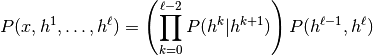
（1） $P(x, h^1, \ldots, h^{\ell}) = \left(\prod_{k=0}^{\ell-2} P(h^k|h^{k+1})\right) P(h^{\ell-1},h^{\ell})$

其中 $x=h^0$ ， $P(h^{k-1} | h^k)$ 是在级别 $k$ 处以RBM的隐藏单位为条件的可见单位的条件分布，并且 $P(h^{\ell-1}, h^{\ell})$ 是顶级中的可见 - 隐藏关节分布RBM。如下图所示。

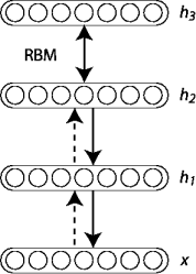
贪婪层级无监督训练的原理可以应用于具有RBM作为每层[Hinton06]，[Bengio07]的构建块的DBN。过程如下：

1. 将第一层训练为RBM，将原始输入 $x = h^{(0)}$ 建模为其可见层。

2. 使用该第一层获得将用作第二层的数据的输入的表示。存在两种常见的解决方案。该表示可以选择为平均激活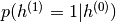 $p(h^{(1)}=1|h^{(0)})$ 或 $p(h^{(1)}|h^{(0)})$ 的样本。

3. 将第二层训练为RBM，将变换后的数据（样本或平均激活）作为训练样本（对于RBM的可见层）。

4. 迭代（2和3）所需数量的层，每次向上传播样本或平均值。

5. 针对DBN对数似然的代理或关于监督的训练标准（在添加额外的学习机制以将学习的表示转换为监督的预测，例如线性分类器）之后微调该深架构的所有参数，。

在本教程中，我们专注于通过监督梯度下降进行微调。具体来说，我们使用逻辑回归分类器，根据DBN的最后一个隐藏层 $h^{(l)}$ 的输出对输入 $x$ 进行分类。然后通过负对数似然成本函数的监督梯度下降来执行微调。由于监督梯度对于每个层的权重和隐藏层偏差只是非零（即对于每个RBM的可见偏差为零），所以该过程等同于用权重和隐层偏差初始化深MLP的参数获得无监督训练策略。

Justifying Greedy-Layer Wise Pre-Training¶

为什么这样的算法工作？例如，具有隐藏层 $h^{(1)}$ 和 $h^{(2)}$ （具有相应的权重参数 $W^{(1)}$ 和 $W^{(2)}$ ），[Hinton06]的2层DBN建立详细推导）， $\log p(x)$ 可以重写为，

（2） $\log p(x) = &KL(Q(h^{(1)}|x)||p(h^{(1)}|x)) + H_{Q(h^{(1)}|x)} + \\ &\sum_h Q(h^{(1)}|x)(\log p(h^{(1)}) + \log p(x|h^{(1)})).$

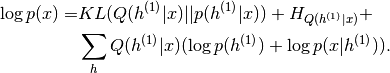
$KL(Q(h^{(1)}|x) || p(h^{(1)}|x))$ 表示如果第一RBM是独立的则第一RBM的后验 $Q(h^{(1)}|x)$ 与同一层的但是由整个DBN定义的概率 $p(h^{(1)}|x)$ 之间的KL散度（即，考虑先前 $p(h^{(1)},h^{(2)})$ 由顶级RBM定义）。 $H_{Q(h^{(1)}|x)}$ 是分布 $Q(h^{(1)}|x)$ 的熵。

可以表明，如果我们初始化两个隐藏层，使得 $W^{(2)}={W^{(1)}}^T$ ， $Q(h^{(1)}|x)=p(h^{(1)}|x)$ 和KL散度项为null。如果我们学习第一级RBM，然后保持其参数 $W^{(1)}$ 固定，则优化等式。（2）相对于 $W^{(2)}$ 可以因此仅增加似然性 $p(x)$ 。

另外，注意如果我们隔离只依赖于 $W^{(2)}$ 的条件，我们得到：

$\sum_h Q(h^{(1)}|x)p(h^{(1)})$

当从第一RBM的训练分布采样 $x$ 时，相对于 $W^{(2)}$ 优化这个值相当于训练第二阶段RBM，使用 $Q(h^{(1)}|x)$ 的输出作为训练分布。

Implementation¶

要在Theano中实现DBN，我们将使用Restricted Boltzmann Machines (RBM)教程中定义的类。还可以观察到DBN的代码与用于SdA的代码非常相似，因为它们都涉及无监督的层级预训练的原理，随后是作为深MLP的监督微调。主要区别是我们使用RBM类而不是dA类。

我们首先定义DBN类，它将存储MLP的层及其相关的RBM。由于我们考虑使用RBM初始化MLP的观点，代码将通过尽可能多地分离用于初始化网络的RBM和用于分类的MLP来反映这一点。

class DBN(object):
    """Deep Belief Network

    A deep belief network is obtained by stacking several RBMs on top of each
    other. The hidden layer of the RBM at layer `i` becomes the input of the
    RBM at layer `i+1`. The first layer RBM gets as input the input of the
    network, and the hidden layer of the last RBM represents the output. When
    used for classification, the DBN is treated as a MLP, by adding a logistic
    regression layer on top.
    """

    def __init__(self, numpy_rng, theano_rng=None, n_ins=784,
                 hidden_layers_sizes=[500, 500], n_outs=10):
        """This class is made to support a variable number of layers.

        :type numpy_rng: numpy.random.RandomState
        :param numpy_rng: numpy random number generator used to draw initial
                    weights

        :type theano_rng: theano.tensor.shared_randomstreams.RandomStreams
        :param theano_rng: Theano random generator; if None is given one is
                           generated based on a seed drawn from `rng`

        :type n_ins: int
        :param n_ins: dimension of the input to the DBN

        :type hidden_layers_sizes: list of ints
        :param hidden_layers_sizes: intermediate layers size, must contain
                               at least one value

        :type n_outs: int
        :param n_outs: dimension of the output of the network
        """

        self.sigmoid_layers = []
        self.rbm_layers = []
        self.params = []
        self.n_layers = len(hidden_layers_sizes)

        assert self.n_layers > 0

        if not theano_rng:
            theano_rng = MRG_RandomStreams(numpy_rng.randint(2 ** 30))

        # allocate symbolic variables for the data

        # the data is presented as rasterized images
        self.x = T.matrix('x')

        # the labels are presented as 1D vector of [int] labels
        self.y = T.ivector('y')

self.sigmoid_layers将存储一起形成MLP的前馈图，而self.rbm_layers将存储用于预训练MLP的每层的RBM。

下一步，我们构建n_layers Sigmoid图层（我们使用Multilayer Perceptron中引入的HiddenLayer类，从tanh到对数函数 $s(x) = \frac{1}{1+e^{-x}}$ ）和n_layers RBM的非线性，其中n_layers是我们模型的深度。我们链接S形层使得它们形成MLP，并且构造每个RBM，使得它们与其对应的S形层共享权重矩阵和隐藏偏差。

        for i in range(self.n_layers):
            # construct the sigmoidal layer

            # the size of the input is either the number of hidden
            # units of the layer below or the input size if we are on
            # the first layer
            if i == 0:
                input_size = n_ins
            else:
                input_size = hidden_layers_sizes[i - 1]

            # the input to this layer is either the activation of the
            # hidden layer below or the input of the DBN if you are on
            # the first layer
            if i == 0:
                layer_input = self.x
            else:
                layer_input = self.sigmoid_layers[-1].output

            sigmoid_layer = HiddenLayer(rng=numpy_rng,
                                        input=layer_input,
                                        n_in=input_size,
                                        n_out=hidden_layers_sizes[i],
                                        activation=T.nnet.sigmoid)

            # add the layer to our list of layers
            self.sigmoid_layers.append(sigmoid_layer)

            # its arguably a philosophical question...  but we are
            # going to only declare that the parameters of the
            # sigmoid_layers are parameters of the DBN. The visible
            # biases in the RBM are parameters of those RBMs, but not
            # of the DBN.
            self.params.extend(sigmoid_layer.params)

            # Construct an RBM that shared weights with this layer
            rbm_layer = RBM(numpy_rng=numpy_rng,
                            theano_rng=theano_rng,
                            input=layer_input,
                            n_visible=input_size,
                            n_hidden=hidden_layers_sizes[i],
                            W=sigmoid_layer.W,
                            hbias=sigmoid_layer.b)
            self.rbm_layers.append(rbm_layer)

剩下的就是堆叠最后一个逻辑回归层，以形成MLP。我们将使用Classifying MNIST digits using Logistic Regression中介绍的LogisticRegression类。

        self.logLayer = LogisticRegression(
            input=self.sigmoid_layers[-1].output,
            n_in=hidden_layers_sizes[-1],
            n_out=n_outs)
        self.params.extend(self.logLayer.params)

        # compute the cost for second phase of training, defined as the
        # negative log likelihood of the logistic regression (output) layer
        self.finetune_cost = self.logLayer.negative_log_likelihood(self.y)

        # compute the gradients with respect to the model parameters
        # symbolic variable that points to the number of errors made on the
        # minibatch given by self.x and self.y
        self.errors = self.logLayer.errors(self.y)

该类还提供了为每个RBM生成训练函数的方法。它们作为列表返回，其中元素 $i$ 是对层 $i$ 处的RBM实现一个训练步骤的函数。

    def pretraining_functions(self, train_set_x, batch_size, k):
        '''Generates a list of functions, for performing one step of
        gradient descent at a given layer. The function will require
        as input the minibatch index, and to train an RBM you just
        need to iterate, calling the corresponding function on all
        minibatch indexes.

        :type train_set_x: theano.tensor.TensorType
        :param train_set_x: Shared var. that contains all datapoints used
                            for training the RBM
        :type batch_size: int
        :param batch_size: size of a [mini]batch
        :param k: number of Gibbs steps to do in CD-k / PCD-k

        '''

        # index to a [mini]batch
        index = T.lscalar('index')  # index to a minibatch

为了能够在训练期间改变学习速率，我们将具有默认值的Theano变量关联到它。

        learning_rate = T.scalar('lr')  # learning rate to use

        # begining of a batch, given `index`
        batch_begin = index * batch_size
        # ending of a batch given `index`
        batch_end = batch_begin + batch_size

        pretrain_fns = []
        for rbm in self.rbm_layers:

            # get the cost and the updates list
            # using CD-k here (persisent=None) for training each RBM.
            # TODO: change cost function to reconstruction error
            cost, updates = rbm.get_cost_updates(learning_rate,
                                                 persistent=None, k=k)

            # compile the theano function
            fn = theano.function(
                inputs=[index, theano.In(learning_rate, value=0.1)],
                outputs=cost,
                updates=updates,
                givens={
                    self.x: train_set_x[batch_begin:batch_end]
                }
            )
            # append `fn` to the list of functions
            pretrain_fns.append(fn)

        return pretrain_fns

现在任何函数pretrain_fns[i]接受参数index和可选lr - 学习速率。注意，参数的名称是构造时给予Theano变量（例如lr）的名称，而不是python变量的名称（例如learning_rate）。在使用Theano时记住这一点。或者，如果您提供k（在CD或PCD中执行的Gibbs步骤数），这也将成为函数的参数。

以相同的方式，DBN类包括用于构建微调所需的函数的方法（train_model，validate_model和test_model函数）。

    def build_finetune_functions(self, datasets, batch_size, learning_rate):
        '''Generates a function `train` that implements one step of
        finetuning, a function `validate` that computes the error on a
        batch from the validation set, and a function `test` that
        computes the error on a batch from the testing set

        :type datasets: list of pairs of theano.tensor.TensorType
        :param datasets: It is a list that contain all the datasets;
                        the has to contain three pairs, `train`,
                        `valid`, `test` in this order, where each pair
                        is formed of two Theano variables, one for the
                        datapoints, the other for the labels
        :type batch_size: int
        :param batch_size: size of a minibatch
        :type learning_rate: float
        :param learning_rate: learning rate used during finetune stage

        '''

        (train_set_x, train_set_y) = datasets[0]
        (valid_set_x, valid_set_y) = datasets[1]
        (test_set_x, test_set_y) = datasets[2]

        # compute number of minibatches for training, validation and testing
        n_valid_batches = valid_set_x.get_value(borrow=True).shape[0]
        n_valid_batches //= batch_size
        n_test_batches = test_set_x.get_value(borrow=True).shape[0]
        n_test_batches //= batch_size

        index = T.lscalar('index')  # index to a [mini]batch

        # compute the gradients with respect to the model parameters
        gparams = T.grad(self.finetune_cost, self.params)

        # compute list of fine-tuning updates
        updates = []
        for param, gparam in zip(self.params, gparams):
            updates.append((param, param - gparam * learning_rate))

        train_fn = theano.function(
            inputs=[index],
            outputs=self.finetune_cost,
            updates=updates,
            givens={
                self.x: train_set_x[
                    index * batch_size: (index + 1) * batch_size
                ],
                self.y: train_set_y[
                    index * batch_size: (index + 1) * batch_size
                ]
            }
        )

        test_score_i = theano.function(
            [index],
            self.errors,
            givens={
                self.x: test_set_x[
                    index * batch_size: (index + 1) * batch_size
                ],
                self.y: test_set_y[
                    index * batch_size: (index + 1) * batch_size
                ]
            }
        )

        valid_score_i = theano.function(
            [index],
            self.errors,
            givens={
                self.x: valid_set_x[
                    index * batch_size: (index + 1) * batch_size
                ],
                self.y: valid_set_y[
                    index * batch_size: (index + 1) * batch_size
                ]
            }
        )

        # Create a function that scans the entire validation set
        def valid_score():
            return [valid_score_i(i) for i in range(n_valid_batches)]

        # Create a function that scans the entire test set
        def test_score():
            return [test_score_i(i) for i in range(n_test_batches)]

        return train_fn, valid_score, test_score

注意，返回的valid_score和test_score不是Theano函数，而是Python函数。这些循环遍及整个验证集和整个测试集，以产生在这些集上获得的损失的列表。

Putting it all together¶

下面的几行代码构造了深信仰网络：

    numpy_rng = numpy.random.RandomState(123)
    print('... building the model')
    # construct the Deep Belief Network
    dbn = DBN(numpy_rng=numpy_rng, n_ins=28 * 28,
              hidden_layers_sizes=[1000, 1000, 1000],
              n_outs=10)

在训练这个网络有两个阶段：（1）逐层预训练和（2）微调阶段。

对于预训练阶段，我们在网络的所有层上循环。对于每个层，我们使用编译的aano函数，其确定到i该函数应用于由pretraining_epochs给出的固定数目的历元的训练集。

    #########################
    # PRETRAINING THE MODEL #
    #########################
    print('... getting the pretraining functions')
    pretraining_fns = dbn.pretraining_functions(train_set_x=train_set_x,
                                                batch_size=batch_size,
                                                k=k)

    print('... pre-training the model')
    start_time = timeit.default_timer()
    # Pre-train layer-wise
    for i in range(dbn.n_layers):
        # go through pretraining epochs
        for epoch in range(pretraining_epochs):
            # go through the training set
            c = []
            for batch_index in range(n_train_batches):
                c.append(pretraining_fns[i](index=batch_index,
                                            lr=pretrain_lr))
            print('Pre-training layer %i, epoch %d, cost ' % (i, epoch), end=' ')
            print(numpy.mean(c, dtype='float64'))

    end_time = timeit.default_timer()

微调循环与Multilayer Perceptron教程中的微调循环非常相似，唯一的区别是我们现在使用build_finetune_functions给出的函数。

Running the Code¶

用户可以通过调用以下代码来运行代码：

python code/DBN.py

使用默认参数，代码运行100个具有大小为10的小批量的训练时期。这对应于执行500,000个无人监督的参数更新。我们使用无监督学习率为0.01，监督学习率为0.1。DBN本身由三层隐藏层组成，每层有1000个单元。在早期停止时，这种配置实现了1.27的最小验证误差，在46个监督时期之后，相应的测试误差为1.34。

在运行在2.80GHz的Intel Xeon（R）X5560 CPU上，使用多线程MKL库（运行在4核上），预训练花费615分钟，平均为2.05分钟/（layer * epoch）。微调仅需101分钟或约2.20分钟/时期。

通过优化验证误差选择超参数。我们测试 $\{10^{-1}, ..., 10^{-5}\}$ 中的无监督学习速率和 $\{10^{-1}, ..., 10^{-4}\}$ 中的监督学习速率。除了早期停止之外，我们没有使用任何形式的正则化，也没有优化预训练的次数。

提示和技巧¶

One way to improve the running time of your code (given that you have sufficient memory available), is to compute the representation of the entire dataset at layer i in a single pass, once the weights of the $i-1$ -th layers have been fixed. 也就是说，首先训练你的第一层RBM。一旦它被训练，你可以计算数据集中每个示例的隐藏单位值，并将其存储为用于训练第二层RBM的新数据集。一旦你训练了第2层的RBM，你以类似的方式计算第3层的数据集等等。这避免了以增加的内存使用为代价计算中间（隐藏层）表示，pretraining_epochs时间。

目录

上一主题

下一主题

这一页

Deep Belief Networks¶

Deep Belief Networks¶

Justifying Greedy-Layer Wise Pre-Training¶

Implementation¶

Putting it all together¶

Running the Code¶

提示和技巧¶