受限玻尔兹曼机(RBM)
注意
本节假设读者已经阅读过使用逻辑回归分析MNIST数字和多层感知器。此外,它使用以下Theano函数和概念:T.tanh、共享变量、基本算术操作、T.grad、随机数、floatX和scan。如果你打算在GPU上运行代码还需阅读GPU。
注意
此部分的代码可从此处下载。
基于能量的模型(EBM)
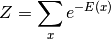
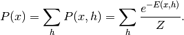
基于能量的模型将标量能量与感兴趣的变量的每个配置相关联。修改能量函数并进行对应的学习,使得其形状具有期望的性质。例如,我们希望似是而非的或期望的配置具有低能量。基于能量的概率模型通过能量函数定义概率分布,如下:
(1)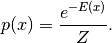
通过与物理系统类比,归一化因子 被称为分割函数。
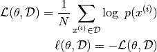
基于能量的模型可以通过对训练数据的经验负对数似然执行(随机)梯度下降来学习。和逻辑回归一样,我们首先定义对数似然,然后将损失函数定义为负对数似然。
使用随机梯度 ,其中
,其中 是模型的参数。
具有隐藏单元的EBMs
在许多感兴趣的情况下,我们不完全观察样本 ,或者我们想引入一些未观察到的变量来增加模型的表达力。因此,我们考虑一个观察到部分(这里仍然表示为)和一个隐藏的部分
 。我们可以写:
(2)
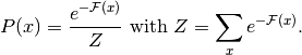
在这种情况下,为了将该公式映射到类似于公式(1),我们引入自由能的符号(来自物理学),定义如下:
(3)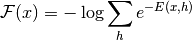
这允许我们写成,
然后,数据负对数似然梯度具有特别有趣的形式。
(4)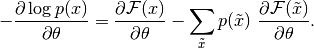
注意,上述梯度包含两个术语,称为正相和负相。术语正相和负相不是指方程中每个术语的符号,而是反映它们对由模型定义的概率密度的影响。第一项增加训练数据的概率(通过减少相应的自由能),而第二项减少由模型产生的样本的概率。
通常难以从分析上确定该梯度,因为其涉及![E_P [ \frac{\partial \mathcal{F}(x)} {\partial \theta} ]](_images/math/b5790ce9ba4f246cfd12e729451ac631f2b7d4ac.png) 的计算。这是对输入(在由模型形成的分布
的计算。这是对输入(在由模型形成的分布 下)的所有可能配置的期望。
使该计算易于处理的第一步是使用固定数量的模型样本来估计期望值。用于估计负相位梯度的样品称为负颗粒,表示为 。梯度可以写成:
(5)
其中我们理想地根据采样的元素 (即,我们正在进行蒙特卡罗)。使用上面的公式,我们几乎有一个实用的随机算法用于学习EBM。唯一缺失的成分是如何提取这些负性颗粒。虽然统计文献中有很多采样方法,但是Markov Chain Monte Carlo方法特别适用于诸如受限玻尔兹曼机(RBM)这样的模型,RBM是一种特定类型的EBM。
受限玻尔兹曼机(RBM)
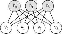
玻尔兹曼机器(BM)是对数线性马尔科夫随机场(MRF)的特定形式,即,其能量函数在其自由参数中是线性的。为了使它们足够强大以表示复杂的分布(即,从有限的参数设置到非参数设置),我们认为一些变量从来没有被观察到(它们被称为隐藏)。通过具有更多的隐藏变量(也称为隐藏单元),我们可以增加玻尔兹曼机(BM)的建模能力。受限玻尔兹曼机进一步限制BM为那些没有可见—可见和隐藏—隐藏连接的BM。RBM的图形描述如下所示。
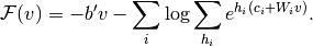
RBM的能量函数 定义为:
定义为:
(6)
其中 表示连接隐藏和可见单元位的权重,
 、
、 分别是可见层和隐藏层的偏移。
这直接转换为以下自由能公式:
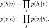
由于RBM的特定结构,可见单元和隐藏单元有条件地彼此独立。使用这个属性,我们可以写成:
二元RBM
在通常研究的使用二元单元(其中 和
和 )的情况下,我们从方程(6)和(2)得到通常神经元激活函数的概率性版本:
(7)
(8)
具有二元单元的RBM的自由能进一步简化为:
(9)
更新带二元单元的方程
组合方程与(5)和(9),我们获得具有二元单元的RBM的以下对数似然梯度:
(10)![- \frac{\partial{ \log p(v)}}{\partial W_{ij}} &=
E_v[p(h_i|v) \cdot v_j]
- v^{(i)}_j \cdot sigm(W_i \cdot v^{(i)} + c_i) \\
-\frac{\partial{ \log p(v)}}{\partial c_i} &=
E_v[p(h_i|v)] - sigm(W_i \cdot v^{(i)}) \\
-\frac{\partial{ \log p(v)}}{\partial b_j} &=
E_v[p(v_j|h)] - v^{(i)}_j](_images/math/712eca5eb5d241fe1dedce7ebb8f59922f9bf258.png)
对于这些方程的更详细的推导,我们推荐读者阅读以下页面或学习AI深度架构的第5节。然而,我们不使用这些公式,而是根据公式(4)使用Theano T.grad获得梯度。
RBM中的采样
 的样本可以通过运行马尔科夫链来收敛,使用Gibbs采样作为过渡算子来获得。
通过具有形式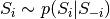 的N个采样子步骤的序列来完成N个随机变量
 的联合的吉布斯采样,其中
 包含
包含 中的
中的 其他随机变量,不包括
 。
。
对于RBM,由可见和隐藏单元的集合组成。然而,由于它们是条件独立的,因此可以执行块吉布斯采样。在此设置中,在给定隐藏单位的固定值的情况下,同时对可见单位进行采样。类似地,隐藏单元在给出可见度的同时被采样。马可夫链中的步骤因此如下:
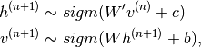
其中 是指在马尔科夫链的第n步的所有隐藏单元的集合。What it means is that, for example,
  is randomly chosen to be 1 (versus 0) with probability
 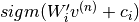 , and similarly,
  is randomly chosen to be 1 (versus 0) with probability
 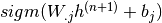 .
.
这可以图形说明:
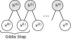
因为 ,样本
,样本 被保证为
被保证为 的精确样本。
理论上,学习过程中的每个参数更新都需要运行一个这样的链来收敛。不用说,这样做将是非常昂贵的。因此,已经为RBM设计了几种算法,以便在学习过程期间从有效地采样。
Contrastive Divergence (CD-k)
对比发散使用两个技巧加速抽样过程:
- 因为我们最终希望
 (数据的真实的底层分布),我们用训练示例初始化马尔可夫链(即,从预期接近
 的分布中,使得链将已经接近已经收敛到其最终分布)。
 - CD不等待链收敛。仅在k-步骤的吉布斯取样之后获得样品。在实践中,
 已经显示出非常好的效果。
Persistent CD
持久性CD [Tieleman08]使用另一个近似值来对进行采样。它依赖于单个马尔可夫链,其具有持久状态(即,不为每个观察到的示例重新启动链)。对于每个参数更新,我们通过简单地运行k-步骤的链来提取新的样本。然后保留链的状态用于随后的更新。
一般的直觉是,如果参数更新与链的混合速率相比足够小,则马尔可夫链应该能够“赶上”模型中的变化。
实现
我们构造一个RBM类。网络的参数可以由构造函数初始化或作为参数传递。当RBM用作深度网络的构造块时,该选项是有用的,在这种情况下,权重矩阵和隐藏层偏置与MLP网络的相应S形层共享。
class RBM(object):
    """Restricted Boltzmann Machine (RBM)  """
    def __init__(
        self,
        input=None,
        n_visible=784,
        n_hidden=500,
        W=None,
        hbias=None,
        vbias=None,
        numpy_rng=None,
        theano_rng=None
    ):
        """
        RBM constructor. Defines the parameters of the model along with
        basic operations for inferring hidden from visible (and vice-versa),
        as well as for performing CD updates.

        :param input: None for standalone RBMs or symbolic variable if RBM is
        part of a larger graph.

        :param n_visible: number of visible units

        :param n_hidden: number of hidden units

        :param W: None for standalone RBMs or symbolic variable pointing to a
        shared weight matrix in case RBM is part of a DBN network; in a DBN,
        the weights are shared between RBMs and layers of a MLP

        :param hbias: None for standalone RBMs or symbolic variable pointing
        to a shared hidden units bias vector in case RBM is part of a
        different network

        :param vbias: None for standalone RBMs or a symbolic variable
        pointing to a shared visible units bias
        """

        self.n_visible = n_visible
        self.n_hidden = n_hidden

        if numpy_rng is None:
            # create a number generator
            numpy_rng = numpy.random.RandomState(1234)

        if theano_rng is None:
            theano_rng = RandomStreams(numpy_rng.randint(2 ** 30))

        if W is None:
            # W is initialized with `initial_W` which is uniformely
            # sampled from -4*sqrt(6./(n_visible+n_hidden)) and
            # 4*sqrt(6./(n_hidden+n_visible)) the output of uniform if
            # converted using asarray to dtype theano.config.floatX so
            # that the code is runable on GPU
            initial_W = numpy.asarray(
                numpy_rng.uniform(
                    low=-4 * numpy.sqrt(6. / (n_hidden + n_visible)),
                    high=4 * numpy.sqrt(6. / (n_hidden + n_visible)),
                    size=(n_visible, n_hidden)
                ),
                dtype=theano.config.floatX
            )
            # theano shared variables for weights and biases
            W = theano.shared(value=initial_W, name='W', borrow=True)

        if hbias is None:
            # create shared variable for hidden units bias
            hbias = theano.shared(
                value=numpy.zeros(
                    n_hidden,
                    dtype=theano.config.floatX
                ),
                name='hbias',
                borrow=True
            )

        if vbias is None:
            # create shared variable for visible units bias
            vbias = theano.shared(
                value=numpy.zeros(
                    n_visible,
                    dtype=theano.config.floatX
                ),
                name='vbias',
                borrow=True
            )

        # initialize input layer for standalone RBM or layer0 of DBN
        self.input = input
        if not input:
            self.input = T.matrix('input')

        self.W = W
        self.hbias = hbias
        self.vbias = vbias
        self.theano_rng = theano_rng
        # **** WARNING: It is not a good idea to put things in this list
        # other than shared variables created in this function.
        self.params = [self.W, self.hbias, self.vbias]
下一步是定义构建与方程相关联的符号图的函数。(7) - (8)。代码如下:
    def propup(self, vis):
        '''This function propagates the visible units activation upwards to
        the hidden units

        Note that we return also the pre-sigmoid activation of the
        layer. As it will turn out later, due to how Theano deals with
        optimizations, this symbolic variable will be needed to write
        down a more stable computational graph (see details in the
        reconstruction cost function)

        '''
        pre_sigmoid_activation = T.dot(vis, self.W) + self.hbias
        return [pre_sigmoid_activation, T.nnet.sigmoid(pre_sigmoid_activation)]
    def sample_h_given_v(self, v0_sample):
        ''' This function infers state of hidden units given visible units '''
        # compute the activation of the hidden units given a sample of
        # the visibles
        pre_sigmoid_h1, h1_mean = self.propup(v0_sample)
        # get a sample of the hiddens given their activation
        # Note that theano_rng.binomial returns a symbolic sample of dtype
        # int64 by default. If we want to keep our computations in floatX
        # for the GPU we need to specify to return the dtype floatX
        h1_sample = self.theano_rng.binomial(size=h1_mean.shape,
                                             n=1, p=h1_mean,
                                             dtype=theano.config.floatX)
        return [pre_sigmoid_h1, h1_mean, h1_sample]
    def propdown(self, hid):
        '''This function propagates the hidden units activation downwards to
        the visible units

        Note that we return also the pre_sigmoid_activation of the
        layer. As it will turn out later, due to how Theano deals with
        optimizations, this symbolic variable will be needed to write
        down a more stable computational graph (see details in the
        reconstruction cost function)

        '''
        pre_sigmoid_activation = T.dot(hid, self.W.T) + self.vbias
        return [pre_sigmoid_activation, T.nnet.sigmoid(pre_sigmoid_activation)]
    def sample_v_given_h(self, h0_sample):
        ''' This function infers state of visible units given hidden units '''
        # compute the activation of the visible given the hidden sample
        pre_sigmoid_v1, v1_mean = self.propdown(h0_sample)
        # get a sample of the visible given their activation
        # Note that theano_rng.binomial returns a symbolic sample of dtype
        # int64 by default. If we want to keep our computations in floatX
        # for the GPU we need to specify to return the dtype floatX
        v1_sample = self.theano_rng.binomial(size=v1_mean.shape,
                                             n=1, p=v1_mean,
                                             dtype=theano.config.floatX)
        return [pre_sigmoid_v1, v1_mean, v1_sample]
然后,我们可以使用这些函数来定义吉布斯采样步骤的符号图。我们定义了两个函数:
gibbs_vhv其执行从可见单位开始的吉布斯采样的步骤。我们将看到,这将有助于从RBM抽样。gibbs_hvh其执行从隐藏单元开始的吉布斯采样的步骤。此功能对于执行CD和PCD更新非常有用。
代码如下:
    def gibbs_hvh(self, h0_sample):
        ''' This function implements one step of Gibbs sampling,
            starting from the hidden state'''
        pre_sigmoid_v1, v1_mean, v1_sample = self.sample_v_given_h(h0_sample)
        pre_sigmoid_h1, h1_mean, h1_sample = self.sample_h_given_v(v1_sample)
        return [pre_sigmoid_v1, v1_mean, v1_sample,
                pre_sigmoid_h1, h1_mean, h1_sample]
    def gibbs_vhv(self, v0_sample):
        ''' This function implements one step of Gibbs sampling,
            starting from the visible state'''
        pre_sigmoid_h1, h1_mean, h1_sample = self.sample_h_given_v(v0_sample)
        pre_sigmoid_v1, v1_mean, v1_sample = self.sample_v_given_h(h1_sample)
        return [pre_sigmoid_h1, h1_mean, h1_sample,
                pre_sigmoid_v1, v1_mean, v1_sample]
注意,我们也返回前S形激活。要理解为什么这是你需要了解一点关于Theano如何工作。每当你编译一个Theano函数,你传递的计算图作为输入获得优化的速度和稳定性。这是通过用其他人改变子图的几个部分来完成的。一个这样的优化表示在softplus方面的形式log(sigmoid(x))的项。我们需要对于交叉熵的这种优化,因为大于30的数字的sigmoid。(或者甚至小于)转到1.和小于-30的数字。转为0,这将强制theano计算log(0),因此我们将获得-inf或NaN作为成本。如果值用softplus表示,我们不会得到这种不良行为。这种优化通常工作正常,但在这里我们有一个特殊的情况。Sigmoid应用于扫描op内部,而日志在外部。因此,Theano只会看到log(scan(..))而不是log(sigmoid(..)),并且不会应用所需的优化。我们不能在扫描中用别的东西替换Sigmoid,因为这只需要在最后一步完成。因此,最简单和更有效的方法是获得pre-Sigmoid激活作为扫描的输出,并应用log和Sigmoid外部扫描,以便Theano可以捕获和优化表达式。
该类还具有计算模型的自由能的函数,其用于计算参数的梯度(参见公式(4))。注意,我们也返回前S形
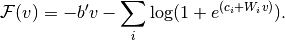
    def free_energy(self, v_sample):
        ''' Function to compute the free energy '''
        wx_b = T.dot(v_sample, self.W) + self.hbias
        vbias_term = T.dot(v_sample, self.vbias)
        hidden_term = T.sum(T.log(1 + T.exp(wx_b)), axis=1)
        return -hidden_term - vbias_term
然后,我们添加一个get_cost_updates方法,其目的是为CD-k和PCD-k更新生成符号渐变。
    def get_cost_updates(self, lr=0.1, persistent=None, k=1):
        """This functions implements one step of CD-k or PCD-k

        :param lr: learning rate used to train the RBM

        :param persistent: None for CD. For PCD, shared variable
            containing old state of Gibbs chain. This must be a shared
            variable of size (batch size, number of hidden units).

        :param k: number of Gibbs steps to do in CD-k/PCD-k

        Returns a proxy for the cost and the updates dictionary. The
        dictionary contains the update rules for weights and biases but
        also an update of the shared variable used to store the persistent
        chain, if one is used.

        """

        # compute positive phase
        pre_sigmoid_ph, ph_mean, ph_sample = self.sample_h_given_v(self.input)

        # decide how to initialize persistent chain:
        # for CD, we use the newly generate hidden sample
        # for PCD, we initialize from the old state of the chain
        if persistent is None:
            chain_start = ph_sample
        else:
            chain_start = persistent
请注意,get_cost_updates将参数作为persistent的变量。这允许我们使用相同的代码来实现CD和PCD。要使用PCD,persistent应该指向一个共享变量,该变量包含来自上一次迭代的Gibbs链的状态。
如果persistent是None,我们用在正相期间生成的隐藏样本来初始化Gibbs链,因此实现CD。一旦我们建立了链的起点,我们就可以计算Gibbs链结束处的样本,我们需要的样本来获得梯度(见公式。(4))。为此,我们将使用Theano提供的scan操作,因此我们敦促读者按照此链接查找它。
        # perform actual negative phase
        # in order to implement CD-k/PCD-k we need to scan over the
        # function that implements one gibbs step k times.
        # Read Theano tutorial on scan for more information :
        # http://deeplearning.net/software/theano/library/scan.html
        # the scan will return the entire Gibbs chain
        (
            [
                pre_sigmoid_nvs,
                nv_means,
                nv_samples,
                pre_sigmoid_nhs,
                nh_means,
                nh_samples
            ],
            updates
        ) = theano.scan(
            self.gibbs_hvh,
            # the None are place holders, saying that
            # chain_start is the initial state corresponding to the
            # 6th output
            outputs_info=[None, None, None, None, None, chain_start],
            n_steps=k,
            name="gibbs_hvh"
        )
一旦我们产生了链,我们在链的末端取样以获得负相的自由能。注意,chain_end是用模型参数表示的符号的Theano变量,如果我们应用T.grad,该函数将尝试通过Gibbs链得到渐变。这不是我们想要的(它会弄乱我们的梯度),因此我们需要向T.grad指示chain_end是一个常数。我们使用T.grad的参数consider_constant来做到这一点。
        # determine gradients on RBM parameters
        # note that we only need the sample at the end of the chain
        chain_end = nv_samples[-1]

        cost = T.mean(self.free_energy(self.input)) - T.mean(
            self.free_energy(chain_end))
        # We must not compute the gradient through the gibbs sampling
        gparams = T.grad(cost, self.params, consider_constant=[chain_end])
最后,我们添加到由scan返回的更新字典(其包含theano_rng的随机状态的更新规则)以包含参数更新。在PCD的情况下,这些也应更新包含Gibbs链的状态的共享变量。
        # constructs the update dictionary
        for gparam, param in zip(gparams, self.params):
            # make sure that the learning rate is of the right dtype
            updates[param] = param - gparam * T.cast(
                lr,
                dtype=theano.config.floatX
            )
        if persistent:
            # Note that this works only if persistent is a shared variable
            updates[persistent] = nh_samples[-1]
            # pseudo-likelihood is a better proxy for PCD
            monitoring_cost = self.get_pseudo_likelihood_cost(updates)
        else:
            # reconstruction cross-entropy is a better proxy for CD
            monitoring_cost = self.get_reconstruction_cost(updates,
                                                           pre_sigmoid_nvs[-1])

        return monitoring_cost, updates
跟踪进度
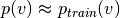
RBM特别难以训练。因为等式(1)的分区函数。(1),我们不能在训练期间估计对数似然性 。因此,我们没有用于选择最佳超参数的直接有用的度量。
用户可以使用几个选项。
检查阴性样品
训练期间获得的负样本可以被可视化。随着训练的进行,我们知道RBM定义的模型更接近真实的底层分布, 。因此,负样本应该看起来像训练集中的样本。显然,错误的超参数可以以这种方式被丢弃。
过滤器的目视检查
通过模型学习的过滤器可以被可视化。这相当于将每个单元的权重绘制为灰度图像(在重新形成到方形矩阵之后)。过滤器应该选择数据中的强特征。虽然不清楚任何数据集,这些功能应该是什么样子,训练在MNIST通常导致过滤器作为行程检测器,而训练自然图像导致Gabor像过滤器,如果训练与稀疏标准。
代理到似然
其他,更易处理的函数可以用作代理的可能性。当使用PCD训练RBM时,可以使用伪似然作为代理。伪似然(PL)计算成本便宜得多,因为它假定所有位都是独立的。因此,
这里 表示除了比特
 之外的的所有比特的集合。因此,log-PL是每个位
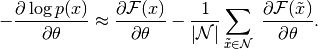
 的对数概率的总和,以所有其他位的状态为条件。对于MNIST,这将涉及对784个输入维度求和,这仍然相当昂贵。为此,我们使用以下随机近似log-PL:
![g = N \cdot \log P(x_i | x_{-i}) \text{, where } i \sim U(0,N), \text{, and}\\
E[ g ] = \log PL(x)](_images/math/2cfd1b83d48af48b58613116a4082a4650db9f73.png)
其中期望是对指数的均匀随机选择,并且 是可见单位的数量。为了与二进制单元一起工作,我们进一步引入符号
 以在位i被翻转(1-> 0,0-> 1)时引用。具有二进制单位的RBM的log-PL然后被写为:
![\log PL(x) &\approx N \cdot \log
\frac {e^{-FE(x)}} {e^{-FE(x)} + e^{-FE(\tilde{x}_i)}} \\
&\approx N \cdot \log[ sigm (FE(\tilde{x}_i) - FE(x)) ]](_images/math/e2477c343b6cd503ab7e7b468be34d0c96d80a3c.png)
因此,我们在RBM类的get_cost_updates函数中返回此成本以及RBM更新。注意,我们修改更新字典以增加位的索引。这将导致位位从所有可能的值 循环,从一个更新到另一个。
注意,对于CD训练,输入和重建之间的交叉熵成本(与用于去噪自动编码器的相同)比伪对数似然更可靠。这里是我们用来计算伪似然的代码:
    def get_pseudo_likelihood_cost(self, updates):
        """Stochastic approximation to the pseudo-likelihood"""

        # index of bit i in expression p(x_i | x_{\i})
        bit_i_idx = theano.shared(value=0, name='bit_i_idx')

        # binarize the input image by rounding to nearest integer
        xi = T.round(self.input)

        # calculate free energy for the given bit configuration
        fe_xi = self.free_energy(xi)

        # flip bit x_i of matrix xi and preserve all other bits x_{\i}
        # Equivalent to xi[:,bit_i_idx] = 1-xi[:, bit_i_idx], but assigns
        # the result to xi_flip, instead of working in place on xi.
        xi_flip = T.set_subtensor(xi[:, bit_i_idx], 1 - xi[:, bit_i_idx])

        # calculate free energy with bit flipped
        fe_xi_flip = self.free_energy(xi_flip)

        # equivalent to e^(-FE(x_i)) / (e^(-FE(x_i)) + e^(-FE(x_{\i})))
        cost = T.mean(self.n_visible * T.log(T.nnet.sigmoid(fe_xi_flip -
                                                            fe_xi)))

        # increment bit_i_idx % number as part of updates
        updates[bit_i_idx] = (bit_i_idx + 1) % self.n_visible

        return cost
主循环
我们现在有所有必要的成分开始训练我们的网络。
然而,在浏览训练循环之前,读者应该熟悉函数tile_raster_images(参见Plotting Samples and Filters)。由于RBM是生成模型,我们有兴趣从中抽样并绘制/可视化这些样本。我们还想要可视化RBM所学到的过滤器(权重),以获得对RBM实际做什么的洞察。但是,请记住,这不提供整个故事,因为我们忽略了偏差,并将权重绘制为乘法常数(权重转换为0和1之间的值)。
具有这些效用函数,我们可以开始训练RBM,并在每个训练时期之后绘制/保存过滤器。我们使用PCD训练RBM,因为它已被证明导致更好的生成模型([Tieleman08])。
    # it is ok for a theano function to have no output
    # the purpose of train_rbm is solely to update the RBM parameters
    train_rbm = theano.function(
        [index],
        cost,
        updates=updates,
        givens={
            x: train_set_x[index * batch_size: (index + 1) * batch_size]
        },
        name='train_rbm'
    )

    plotting_time = 0.
    start_time = timeit.default_timer()

    # go through training epochs
    for epoch in range(training_epochs):

        # go through the training set
        mean_cost = []
        for batch_index in range(n_train_batches):
            mean_cost += [train_rbm(batch_index)]

        print('Training epoch %d, cost is ' % epoch, numpy.mean(mean_cost))

        # Plot filters after each training epoch
        plotting_start = timeit.default_timer()
        # Construct image from the weight matrix
        image = Image.fromarray(
            tile_raster_images(
                X=rbm.W.get_value(borrow=True).T,
                img_shape=(28, 28),
                tile_shape=(10, 10),
                tile_spacing=(1, 1)
            )
        )
        image.save('filters_at_epoch_%i.png' % epoch)
        plotting_stop = timeit.default_timer()
        plotting_time += (plotting_stop - plotting_start)

    end_time = timeit.default_timer()

    pretraining_time = (end_time - start_time) - plotting_time

    print ('Training took %f minutes' % (pretraining_time / 60.))
一旦RBM被训练,我们可以使用gibbs_vhv函数来实现采样所需的Gibbs链。我们从测试示例开始初始化Gibbs链(尽管我们可以从训练集中选择它),以加快收敛并避免随机初始化的问题。我们再次使用Theano的scan op在每次绘图前执行1000个步骤。
    #################################
    #     Sampling from the RBM     #
    #################################
    # find out the number of test samples
    number_of_test_samples = test_set_x.get_value(borrow=True).shape[0]

    # pick random test examples, with which to initialize the persistent chain
    test_idx = rng.randint(number_of_test_samples - n_chains)
    persistent_vis_chain = theano.shared(
        numpy.asarray(
            test_set_x.get_value(borrow=True)[test_idx:test_idx + n_chains],
            dtype=theano.config.floatX
        )
    )
接下来,我们并行创建20个持久链来获取我们的样本。为此,我们编译一个aano函数,它执行一个Gibbs步骤,并用新的可见样本更新持久链的状态。我们对大量步骤迭代应用此函数,以每1000个步骤绘制样本。
    plot_every = 1000
    # define one step of Gibbs sampling (mf = mean-field) define a
    # function that does `plot_every` steps before returning the
    # sample for plotting
    (
        [
            presig_hids,
            hid_mfs,
            hid_samples,
            presig_vis,
            vis_mfs,
            vis_samples
        ],
        updates
    ) = theano.scan(
        rbm.gibbs_vhv,
        outputs_info=[None, None, None, None, None, persistent_vis_chain],
        n_steps=plot_every,
        name="gibbs_vhv"
    )

    # add to updates the shared variable that takes care of our persistent
    # chain :.
    updates.update({persistent_vis_chain: vis_samples[-1]})
    # construct the function that implements our persistent chain.
    # we generate the "mean field" activations for plotting and the actual
    # samples for reinitializing the state of our persistent chain
    sample_fn = theano.function(
        [],
        [
            vis_mfs[-1],
            vis_samples[-1]
        ],
        updates=updates,
        name='sample_fn'
    )

    # create a space to store the image for plotting ( we need to leave
    # room for the tile_spacing as well)
    image_data = numpy.zeros(
        (29 * n_samples + 1, 29 * n_chains - 1),
        dtype='uint8'
    )
    for idx in range(n_samples):
        # generate `plot_every` intermediate samples that we discard,
        # because successive samples in the chain are too correlated
        vis_mf, vis_sample = sample_fn()
        print(' ... plotting sample %d' % idx)
        image_data[29 * idx:29 * idx + 28, :] = tile_raster_images(
            X=vis_mf,
            img_shape=(28, 28),
            tile_shape=(1, n_chains),
            tile_spacing=(1, 1)
        )

    # construct image
    image = Image.fromarray(image_data)
    image.save('samples.png')
结果
我们使用PCD-15,学习率为0.1,批次大小为20,运行代码为15个时代。在英特尔至强E5430 @ 2.66GHz CPU上,使用单线程GotoBLAS,该型号的训练时间为122.466分钟。
输出如下:
... loading data
Training epoch 0, cost is  -90.6507246003
Training epoch 1, cost is  -81.235857373
Training epoch 2, cost is  -74.9120966945
Training epoch 3, cost is  -73.0213216101
Training epoch 4, cost is  -68.4098570497
Training epoch 5, cost is  -63.2693021647
Training epoch 6, cost is  -65.99578971
Training epoch 7, cost is  -68.1236650015
Training epoch 8, cost is  -68.3207365087
Training epoch 9, cost is  -64.2949797113
Training epoch 10, cost is  -61.5194867893
Training epoch 11, cost is  -61.6539369402
Training epoch 12, cost is  -63.5465278086
Training epoch 13, cost is  -63.3787093527
Training epoch 14, cost is  -62.755739271
Training took 122.466000 minutes
 ... plotting sample  0
 ... plotting sample  1
 ... plotting sample  2
 ... plotting sample  3
 ... plotting sample  4
 ... plotting sample  5
 ... plotting sample  6
 ... plotting sample  7
 ... plotting sample  8
 ... plotting sample  9
下面的图片显示15个epoch之后的过滤器:
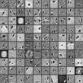
在15个epoch之后获得的过滤器。
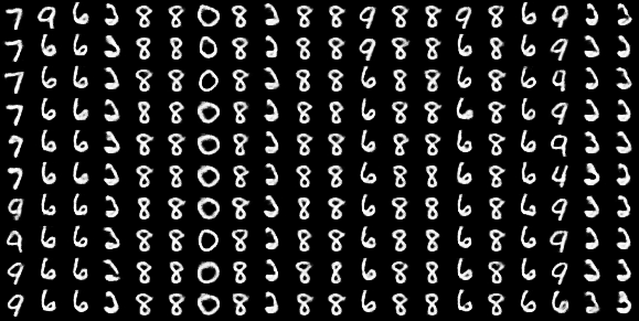
这里是训练后由RBM生成的样本。每行代表一小批阴性颗粒(来自独立的Gibbs链的样品)。在这些行中的每一行之间进行1000步吉布斯取样。