多层感知器¶

注意

本节假设读者已阅读过使用逻辑回归分类MNIST数字。此外，它使用以下新的Theano函数和概念：T.tanh、共享变量、基本算术操作、T.grad、L1和L2正则化、floatX。如果你打算在GPU上运行代码也读取GPU。

注意

此部分的代码可从此处下载。

我们将使用Theano演示的下一个架构是只有一个隐藏层的多层感知器（MLP）。MLP可以被视为逻辑回归分类器，其输入首先使用学习过的非线性变换 $\Phi$ 来转换。此转换将输入数据投影到一个线性可分的空间。该中间层被称为隐藏层。单个隐藏层足以使MLP成为一个广泛的approximator。然而，我们将在后面看到，使用许多这样的隐藏层有很大的好处，例如深度学习的最初的层。请参阅这些课程笔记，了解有关MLP的简介、反向传播算法以及如何训练MLP。

本教程将再次解决MNIST数字分类的问题。

模型¶

具有单个隐藏层的MLP（或人工神经网络-ANN）可以图形表示如下：

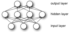
形式上，单隐层MLP是一个函数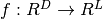 $f: R^D \rightarrow R^L$ ，其中 $D$ 是输入向量 $x$ 的大小、 $L$ 是输出向量 $f(x)$ 的大小，所以用矩阵表示法：

$f(x) = G( b^{(2)} + W^{(2)}( s( b^{(1)} + W^{(1)} x))),$

$b^{(1)}$ 、 $b^{(2)}$ 为偏差向量； $W^{(1)}$ 、 $W^{(2)}$ 为权重矩阵； $G$ 和 $s$ 为激活函数。

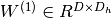向量 $h(x) = \Phi(x) = s(b^{(1)} + W^{(1)} x)$ 构成隐藏层。 $W^{(1)} \in R^{D \times D_h}$ 是连接输入向量与隐藏层的权重矩阵。每列 $W^{(1)}_{\cdot i}$ 表示从输入单元到第i个隐藏单元的权重。 $s$ 的典型选择包括 $tanh$ ， $tanh(a)=(e^a-e^{-a})/(e^a+e^{-a})$ 或逻辑 $sigmoid$ 函数， $sigmoid(a)=1/(1+e^{-a})$ 。在本教程中，我们将使用 $tanh$ ，因为它通常可以获得更快的训练（有时甚至更好的局部最小值）。 $tanh$ 和 $sigmoid$ 都是标量到标量的函数，但是它们扩展到向量和张量时在元素级别上应用它们非常自然（例如，分别在向量的每个元素上应用，将产生相同大小的向量）。

然后获得输出向量为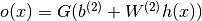： $o(x) = G(b^{(2)} + W^{(2)} h(x))$ 。读者应该认识这个形式，我们已经在使用逻辑回归分类MNIST数字用过它。如前所述，可以通过选择 $G$ 作为 $softmax$ 函数（在多类分类的情况下）获得是否属于某一类别的概率。

为了训练MLP，我们学习模型的所有参数，这里我们使用随机梯度下降和minibatch。要学习的参数集是集合 $\theta = \{W^{(2)},b^{(2)},W^{(1)},b^{(1)}\}$ 。梯度的获得 $\partial{\ell}/\partial{\theta}$ 可以通过反向传播算法（推导的链式规则的特殊情况）来实现。幸运的是，由于Theano执行自动微分，我们不需要在教程中涉及这个！

从逻辑回归到MLP ¶

本教程将重点介绍单隐层MLP。我们首先实现一个代表隐藏层的类。为了构建MLP，我们将只需要在上面抛出一个逻辑回归层。

class HiddenLayer(object):
    def __init__(self, rng, input, n_in, n_out, W=None, b=None,
                 activation=T.tanh):
        """
        Typical hidden layer of a MLP: units are fully-connected and have
        sigmoidal activation function. Weight matrix W is of shape (n_in,n_out)
        and the bias vector b is of shape (n_out,).

        NOTE : The nonlinearity used here is tanh

        Hidden unit activation is given by: tanh(dot(input,W) + b)

        :type rng: numpy.random.RandomState
        :param rng: a random number generator used to initialize weights

        :type input: theano.tensor.dmatrix
        :param input: a symbolic tensor of shape (n_examples, n_in)

        :type n_in: int
        :param n_in: dimensionality of input

        :type n_out: int
        :param n_out: number of hidden units

        :type activation: theano.Op or function
        :param activation: Non linearity to be applied in the hidden
                           layer
        """
        self.input = input

第 $i$ 层隐藏层的权重的初始值应该从一个对称区间均匀地采样，而这个区间依赖于激活函数。对于 $tanh$ 激活函数，[Xavier10]中得到的结果显示区间应为 $[-\sqrt{\frac{6}{fan_{in}+fan_{out}}},\sqrt{\frac{6}{fan_{in}+fan_{out}}}]$ ，其中 $fan_{in}$ 是 $(i-1)$ 层中神经元的数量， $fan_{out}$ 是 $i$ 层中神经元的数量。对于sigmoid函数，区间为 $[-4\sqrt{\frac{6}{fan_{in}+fan_{out}}},4\sqrt{\frac{6}{fan_{in}+fan_{out}}}]$ 。该初始化确保在训练早期，每个神经元在其激活函数的控制下运作，此时信息可以容易地向前（从输入到输出的激活）和向后（从输出到输入的梯度）传播。

        # `W` is initialized with `W_values` which is uniformely sampled
        # from sqrt(-6./(n_in+n_hidden)) and sqrt(6./(n_in+n_hidden))
        # for tanh activation function
        # the output of uniform if converted using asarray to dtype
        # theano.config.floatX so that the code is runable on GPU
        # Note : optimal initialization of weights is dependent on the
        #        activation function used (among other things).
        #        For example, results presented in [Xavier10] suggest that you
        #        should use 4 times larger initial weights for sigmoid
        #        compared to tanh
        #        We have no info for other function, so we use the same as
        #        tanh.
        if W is None:
            W_values = numpy.asarray(
                rng.uniform(
                    low=-numpy.sqrt(6. / (n_in + n_out)),
                    high=numpy.sqrt(6. / (n_in + n_out)),
                    size=(n_in, n_out)
                ),
                dtype=theano.config.floatX
            )
            if activation == theano.tensor.nnet.sigmoid:
                W_values *= 4

            W = theano.shared(value=W_values, name='W', borrow=True)

        if b is None:
            b_values = numpy.zeros((n_out,), dtype=theano.config.floatX)
            b = theano.shared(value=b_values, name='b', borrow=True)

        self.W = W
        self.b = b

注意，我们使用给定的非线性函数作为隐藏层的激活函数。默认情况下，这是tanh，但在许多情况下，我们可能想使用其他的函数。

        lin_output = T.dot(input, self.W) + self.b
        self.output = (
            lin_output if activation is None
            else activation(lin_output)
        )

如果你看看理论，就知道这个类实现计算隐藏层值 $h(x) = \Phi(x) = s(b^{(1)} + W^{(1)} x)$ 的图。如果你将这个图作为在上一教程使用逻辑回归分类MNIST数字中被实现的LogisticRegression类的输入，你就可以得到MLP的输出。你可以在下面的MLP类的简短的实现中看到这一点。

class MLP(object):
    """Multi-Layer Perceptron Class

    A multilayer perceptron is a feedforward artificial neural network model
    that has one layer or more of hidden units and nonlinear activations.
    Intermediate layers usually have as activation function tanh or the
    sigmoid function (defined here by a ``HiddenLayer`` class)  while the
    top layer is a softmax layer (defined here by a ``LogisticRegression``
    class).
    """

    def __init__(self, rng, input, n_in, n_hidden, n_out):
        """Initialize the parameters for the multilayer perceptron

        :type rng: numpy.random.RandomState
        :param rng: a random number generator used to initialize weights

        :type input: theano.tensor.TensorType
        :param input: symbolic variable that describes the input of the
        architecture (one minibatch)

        :type n_in: int
        :param n_in: number of input units, the dimension of the space in
        which the datapoints lie

        :type n_hidden: int
        :param n_hidden: number of hidden units

        :type n_out: int
        :param n_out: number of output units, the dimension of the space in
        which the labels lie

        """

        # Since we are dealing with a one hidden layer MLP, this will translate
        # into a HiddenLayer with a tanh activation function connected to the
        # LogisticRegression layer; the activation function can be replaced by
        # sigmoid or any other nonlinear function
        self.hiddenLayer = HiddenLayer(
            rng=rng,
            input=input,
            n_in=n_in,
            n_out=n_hidden,
            activation=T.tanh
        )

        # The logistic regression layer gets as input the hidden units
        # of the hidden layer
        self.logRegressionLayer = LogisticRegression(
            input=self.hiddenLayer.output,
            n_in=n_hidden,
            n_out=n_out
        )

在本教程中，我们还将使用L1和L2正则化（参见L1和L2正则化）。为此，我们需要计算权重 $W^{(1)}, W^{(2)}$ 的L1范数和L2平方的范数。

        # L1 norm ; one regularization option is to enforce L1 norm to
        # be small
        self.L1 = (
            abs(self.hiddenLayer.W).sum()
            + abs(self.logRegressionLayer.W).sum()
        )

        # square of L2 norm ; one regularization option is to enforce
        # square of L2 norm to be small
        self.L2_sqr = (
            (self.hiddenLayer.W ** 2).sum()
            + (self.logRegressionLayer.W ** 2).sum()
        )

        # negative log likelihood of the MLP is given by the negative
        # log likelihood of the output of the model, computed in the
        # logistic regression layer
        self.negative_log_likelihood = (
            self.logRegressionLayer.negative_log_likelihood
        )
        # same holds for the function computing the number of errors
        self.errors = self.logRegressionLayer.errors

        # the parameters of the model are the parameters of the two layer it is
        # made out of
        self.params = self.hiddenLayer.params + self.logRegressionLayer.params

如前所述，我们使用随机梯度下降与mini-batch训练这个模型。不同的是，我们修改cost函数使其包含正则化项。L1_reg和L2_reg是控制总cost函数中这些正则项的权重的超参数。计算新cost函数的代码是：

    # the cost we minimize during training is the negative log likelihood of
    # the model plus the regularization terms (L1 and L2); cost is expressed
    # here symbolically
    cost = (
        classifier.negative_log_likelihood(y)
        + L1_reg * classifier.L1
        + L2_reg * classifier.L2_sqr
    )

然后，我们使用梯度更新模型的参数。此代码几乎与逻辑回归的代码完全相同。只有参数数量不同。为了解决这个问题（并编写可以用于任意数量参数的代码），我们将使用模型params创建一个参数列表并解析它，然后在每一步计算梯度。

    # compute the gradient of cost with respect to theta (sorted in params)
    # the resulting gradients will be stored in a list gparams
    gparams = [T.grad(cost, param) for param in classifier.params]

    # specify how to update the parameters of the model as a list of
    # (variable, update expression) pairs

    # given two lists of the same length, A = [a1, a2, a3, a4] and
    # B = [b1, b2, b3, b4], zip generates a list C of same size, where each
    # element is a pair formed from the two lists :
    #    C = [(a1, b1), (a2, b2), (a3, b3), (a4, b4)]
    updates = [
        (param, param - learning_rate * gparam)
        for param, gparam in zip(classifier.params, gparams)
    ]

    # compiling a Theano function `train_model` that returns the cost, but
    # in the same time updates the parameter of the model based on the rules
    # defined in `updates`
    train_model = theano.function(
        inputs=[index],
        outputs=cost,
        updates=updates,
        givens={
            x: train_set_x[index * batch_size: (index + 1) * batch_size],
            y: train_set_y[index * batch_size: (index + 1) * batch_size]
        }
    )

合在一起¶

讲述基本概念之后，编写MLP类变得相当容易。下面的代码显示了如何做到这一点，类似于我们以前的logistic回归实现。

"""
This tutorial introduces the multilayer perceptron using Theano.

 A multilayer perceptron is a logistic regressor where
instead of feeding the input to the logistic regression you insert a
intermediate layer, called the hidden layer, that has a nonlinear
activation function (usually tanh or sigmoid) . One can use many such
hidden layers making the architecture deep. The tutorial will also tackle
the problem of MNIST digit classification.

.. math::

    f(x) = G( b^{(2)} + W^{(2)}( s( b^{(1)} + W^{(1)} x))),

References:

    - textbooks: "Pattern Recognition and Machine Learning" -
                 Christopher M. Bishop, section 5

"""

from __future__ import print_function

__docformat__ = 'restructedtext en'


import os
import sys
import timeit

import numpy

import theano
import theano.tensor as T


from logistic_sgd import LogisticRegression, load_data


# start-snippet-1
class HiddenLayer(object):
    def __init__(self, rng, input, n_in, n_out, W=None, b=None,
                 activation=T.tanh):
        """
        Typical hidden layer of a MLP: units are fully-connected and have
        sigmoidal activation function. Weight matrix W is of shape (n_in,n_out)
        and the bias vector b is of shape (n_out,).

        NOTE : The nonlinearity used here is tanh

        Hidden unit activation is given by: tanh(dot(input,W) + b)

        :type rng: numpy.random.RandomState
        :param rng: a random number generator used to initialize weights

        :type input: theano.tensor.dmatrix
        :param input: a symbolic tensor of shape (n_examples, n_in)

        :type n_in: int
        :param n_in: dimensionality of input

        :type n_out: int
        :param n_out: number of hidden units

        :type activation: theano.Op or function
        :param activation: Non linearity to be applied in the hidden
                           layer
        """
        self.input = input
        # end-snippet-1

        # `W` is initialized with `W_values` which is uniformely sampled
        # from sqrt(-6./(n_in+n_hidden)) and sqrt(6./(n_in+n_hidden))
        # for tanh activation function
        # the output of uniform if converted using asarray to dtype
        # theano.config.floatX so that the code is runable on GPU
        # Note : optimal initialization of weights is dependent on the
        #        activation function used (among other things).
        #        For example, results presented in [Xavier10] suggest that you
        #        should use 4 times larger initial weights for sigmoid
        #        compared to tanh
        #        We have no info for other function, so we use the same as
        #        tanh.
        if W is None:
            W_values = numpy.asarray(
                rng.uniform(
                    low=-numpy.sqrt(6. / (n_in + n_out)),
                    high=numpy.sqrt(6. / (n_in + n_out)),
                    size=(n_in, n_out)
                ),
                dtype=theano.config.floatX
            )
            if activation == theano.tensor.nnet.sigmoid:
                W_values *= 4

            W = theano.shared(value=W_values, name='W', borrow=True)

        if b is None:
            b_values = numpy.zeros((n_out,), dtype=theano.config.floatX)
            b = theano.shared(value=b_values, name='b', borrow=True)

        self.W = W
        self.b = b

        lin_output = T.dot(input, self.W) + self.b
        self.output = (
            lin_output if activation is None
            else activation(lin_output)
        )
        # parameters of the model
        self.params = [self.W, self.b]


# start-snippet-2
class MLP(object):
    """Multi-Layer Perceptron Class

    A multilayer perceptron is a feedforward artificial neural network model
    that has one layer or more of hidden units and nonlinear activations.
    Intermediate layers usually have as activation function tanh or the
    sigmoid function (defined here by a ``HiddenLayer`` class)  while the
    top layer is a softmax layer (defined here by a ``LogisticRegression``
    class).
    """

    def __init__(self, rng, input, n_in, n_hidden, n_out):
        """Initialize the parameters for the multilayer perceptron

        :type rng: numpy.random.RandomState
        :param rng: a random number generator used to initialize weights

        :type input: theano.tensor.TensorType
        :param input: symbolic variable that describes the input of the
        architecture (one minibatch)

        :type n_in: int
        :param n_in: number of input units, the dimension of the space in
        which the datapoints lie

        :type n_hidden: int
        :param n_hidden: number of hidden units

        :type n_out: int
        :param n_out: number of output units, the dimension of the space in
        which the labels lie

        """

        # Since we are dealing with a one hidden layer MLP, this will translate
        # into a HiddenLayer with a tanh activation function connected to the
        # LogisticRegression layer; the activation function can be replaced by
        # sigmoid or any other nonlinear function
        self.hiddenLayer = HiddenLayer(
            rng=rng,
            input=input,
            n_in=n_in,
            n_out=n_hidden,
            activation=T.tanh
        )

        # The logistic regression layer gets as input the hidden units
        # of the hidden layer
        self.logRegressionLayer = LogisticRegression(
            input=self.hiddenLayer.output,
            n_in=n_hidden,
            n_out=n_out
        )
        # end-snippet-2 start-snippet-3
        # L1 norm ; one regularization option is to enforce L1 norm to
        # be small
        self.L1 = (
            abs(self.hiddenLayer.W).sum()
            + abs(self.logRegressionLayer.W).sum()
        )

        # square of L2 norm ; one regularization option is to enforce
        # square of L2 norm to be small
        self.L2_sqr = (
            (self.hiddenLayer.W ** 2).sum()
            + (self.logRegressionLayer.W ** 2).sum()
        )

        # negative log likelihood of the MLP is given by the negative
        # log likelihood of the output of the model, computed in the
        # logistic regression layer
        self.negative_log_likelihood = (
            self.logRegressionLayer.negative_log_likelihood
        )
        # same holds for the function computing the number of errors
        self.errors = self.logRegressionLayer.errors

        # the parameters of the model are the parameters of the two layer it is
        # made out of
        self.params = self.hiddenLayer.params + self.logRegressionLayer.params
        # end-snippet-3

        # keep track of model input
        self.input = input


def test_mlp(learning_rate=0.01, L1_reg=0.00, L2_reg=0.0001, n_epochs=1000,
             dataset='mnist.pkl.gz', batch_size=20, n_hidden=500):
    """
    Demonstrate stochastic gradient descent optimization for a multilayer
    perceptron

    This is demonstrated on MNIST.

    :type learning_rate: float
    :param learning_rate: learning rate used (factor for the stochastic
    gradient

    :type L1_reg: float
    :param L1_reg: L1-norm's weight when added to the cost (see
    regularization)

    :type L2_reg: float
    :param L2_reg: L2-norm's weight when added to the cost (see
    regularization)

    :type n_epochs: int
    :param n_epochs: maximal number of epochs to run the optimizer

    :type dataset: string
    :param dataset: the path of the MNIST dataset file from
                 http://www.iro.umontreal.ca/~lisa/deep/data/mnist/mnist.pkl.gz


   """
    datasets = load_data(dataset)

    train_set_x, train_set_y = datasets[0]
    valid_set_x, valid_set_y = datasets[1]
    test_set_x, test_set_y = datasets[2]

    # compute number of minibatches for training, validation and testing
    n_train_batches = train_set_x.get_value(borrow=True).shape[0] // batch_size
    n_valid_batches = valid_set_x.get_value(borrow=True).shape[0] // batch_size
    n_test_batches = test_set_x.get_value(borrow=True).shape[0] // batch_size

    ######################
    # BUILD ACTUAL MODEL #
    ######################
    print('... building the model')

    # allocate symbolic variables for the data
    index = T.lscalar()  # index to a [mini]batch
    x = T.matrix('x')  # the data is presented as rasterized images
    y = T.ivector('y')  # the labels are presented as 1D vector of
                        # [int] labels

    rng = numpy.random.RandomState(1234)

    # construct the MLP class
    classifier = MLP(
        rng=rng,
        input=x,
        n_in=28 * 28,
        n_hidden=n_hidden,
        n_out=10
    )

    # start-snippet-4
    # the cost we minimize during training is the negative log likelihood of
    # the model plus the regularization terms (L1 and L2); cost is expressed
    # here symbolically
    cost = (
        classifier.negative_log_likelihood(y)
        + L1_reg * classifier.L1
        + L2_reg * classifier.L2_sqr
    )
    # end-snippet-4

    # compiling a Theano function that computes the mistakes that are made
    # by the model on a minibatch
    test_model = theano.function(
        inputs=[index],
        outputs=classifier.errors(y),
        givens={
            x: test_set_x[index * batch_size:(index + 1) * batch_size],
            y: test_set_y[index * batch_size:(index + 1) * batch_size]
        }
    )

    validate_model = theano.function(
        inputs=[index],
        outputs=classifier.errors(y),
        givens={
            x: valid_set_x[index * batch_size:(index + 1) * batch_size],
            y: valid_set_y[index * batch_size:(index + 1) * batch_size]
        }
    )

    # start-snippet-5
    # compute the gradient of cost with respect to theta (sorted in params)
    # the resulting gradients will be stored in a list gparams
    gparams = [T.grad(cost, param) for param in classifier.params]

    # specify how to update the parameters of the model as a list of
    # (variable, update expression) pairs

    # given two lists of the same length, A = [a1, a2, a3, a4] and
    # B = [b1, b2, b3, b4], zip generates a list C of same size, where each
    # element is a pair formed from the two lists :
    #    C = [(a1, b1), (a2, b2), (a3, b3), (a4, b4)]
    updates = [
        (param, param - learning_rate * gparam)
        for param, gparam in zip(classifier.params, gparams)
    ]

    # compiling a Theano function `train_model` that returns the cost, but
    # in the same time updates the parameter of the model based on the rules
    # defined in `updates`
    train_model = theano.function(
        inputs=[index],
        outputs=cost,
        updates=updates,
        givens={
            x: train_set_x[index * batch_size: (index + 1) * batch_size],
            y: train_set_y[index * batch_size: (index + 1) * batch_size]
        }
    )
    # end-snippet-5

    ###############
    # TRAIN MODEL #
    ###############
    print('... training')

    # early-stopping parameters
    patience = 10000  # look as this many examples regardless
    patience_increase = 2  # wait this much longer when a new best is
                           # found
    improvement_threshold = 0.995  # a relative improvement of this much is
                                   # considered significant
    validation_frequency = min(n_train_batches, patience // 2)
                                  # go through this many
                                  # minibatche before checking the network
                                  # on the validation set; in this case we
                                  # check every epoch

    best_validation_loss = numpy.inf
    best_iter = 0
    test_score = 0.
    start_time = timeit.default_timer()

    epoch = 0
    done_looping = False

    while (epoch < n_epochs) and (not done_looping):
        epoch = epoch + 1
        for minibatch_index in range(n_train_batches):

            minibatch_avg_cost = train_model(minibatch_index)
            # iteration number
            iter = (epoch - 1) * n_train_batches + minibatch_index

            if (iter + 1) % validation_frequency == 0:
                # compute zero-one loss on validation set
                validation_losses = [validate_model(i) for i
                                     in range(n_valid_batches)]
                this_validation_loss = numpy.mean(validation_losses)

                print(
                    'epoch %i, minibatch %i/%i, validation error %f %%' %
                    (
                        epoch,
                        minibatch_index + 1,
                        n_train_batches,
                        this_validation_loss * 100.
                    )
                )

                # if we got the best validation score until now
                if this_validation_loss < best_validation_loss:
                    #improve patience if loss improvement is good enough
                    if (
                        this_validation_loss < best_validation_loss *
                        improvement_threshold
                    ):
                        patience = max(patience, iter * patience_increase)

                    best_validation_loss = this_validation_loss
                    best_iter = iter

                    # test it on the test set
                    test_losses = [test_model(i) for i
                                   in range(n_test_batches)]
                    test_score = numpy.mean(test_losses)

                    print(('     epoch %i, minibatch %i/%i, test error of '
                           'best model %f %%') %
                          (epoch, minibatch_index + 1, n_train_batches,
                           test_score * 100.))

            if patience <= iter:
                done_looping = True
                break

    end_time = timeit.default_timer()
    print(('Optimization complete. Best validation score of %f %% '
           'obtained at iteration %i, with test performance %f %%') %
          (best_validation_loss * 100., best_iter + 1, test_score * 100.))
    print(('The code for file ' +
           os.path.split(__file__)[1] +
           ' ran for %.2fm' % ((end_time - start_time) / 60.)), file=sys.stderr)


if __name__ == '__main__':
    test_mlp()

然后，用户可以通过调用以下代码来运行代码：

python code/mlp.py

输出应该是以下形式：

Optimization complete. Best validation score of 1.690000 % obtained at iteration 2070000, with test performance 1.650000 %
The code for file mlp.py ran for 97.34m

在Intel(R) Core(TM) i7-2600K CPU @ 3.40GHz上，代码以大约10.3 epoch/分钟运行，并且花费828个epoch以达到1.65％的测试误差。

为了更好地理解这一点，我们将读者引向此页面的结果部分。

训练MLP的提示和技巧¶

在上述代码中有几个超参数，它们不是（并且一般来说不能通过梯度下降来优化）。严格地说，为这些超参数找到一组最优的值不是一个可行的问题。首先，我们不能单独地优化它们中的每一个。第二，我们不能容易地应用我们之前描述的梯度技术（部分是因为一些参数是离散值，而其它的是实值）。第三，优化问题不是凸的，并且找到（局部）最小值将涉及非凡的巨大工作量。

好消息是，在过去25年里，研究人员们想出了各种各样的经验法则用于在神经网络中选择超参数。一份关于这些技巧的非常好的概述可以查看Yann LeCun，Leon Bottou，Genevieve Orr和Klaus-Robert Mueller的Efficient BackProp。在这里，我们总结相同的问题，同时也强调我们在代码实际运用中使用的参数和方法。

非线性函数¶

两个最常见的非线性函数是 $sigmoid$ 和 $tanh$ 函数。由于在第4.4节中解释的原因，优先考虑原点对称的非线性函数，因为它们倾向于对下一层产生均值为零的输入（这是一种期望的性质）。根据经验，我们观察到 $tanh$ 具有更好的收敛性质。

权重初始化¶

在初始化时，我们希望权重围绕原点足够小，使得激活函数在其线性区间中操作，其中梯度是最大的。其它期望的性质，特别是对于深层网络，是保存激活的方差以及从层到层的反向传播梯度的方差。这允许信息在网络中很好地向上和向下流动，并减少层之间的差异。在一些假设下，权衡这两个约束条件，则有以下初始化：tanh函数为 $uniform[-\frac{\sqrt{6}}{\sqrt{fan_{in}+fan_{out}}},\frac{\sqrt{6}}{\sqrt{fan_{in}+fan_{out}}}]$ 和sigmoid函数为 $uniform[-4*\frac{\sqrt{6}}{\sqrt{fan_{in}+fan_{out}}},4*\frac{\sqrt{6}}{\sqrt{fan_{in}+fan_{out}}}]$ 。其中 $fan_{in}$ 是输入单元的数量， $fan_{out}$ 隐藏单元的数量。有关数学方面的讨论，请参阅[Xavier10]。

学习速率¶

有很多关于选择良好的学习率的文献。最简单的解决方案是简单地固定一个速率。经验法则：尝试几个对数间隔值（ $10^{-1},10^{-2},\ldots$ ），并缩小（对数）搜索区间到验证集错误率最低的区域。

有时候，减少学习率是一个好主意。这样做的一个简单规则是 $\frac{\mu_0}{1 + d\times t}$ ，其中 $\mu_0$ 是初始速率（可能使用上述区间搜索方法选定的）， $d$ 是所谓的“减少常数”，其（通常是更小的正数， $10^{-3}$ 或更小）控制着学习速率减小的速率， $t$ 表示epoch/阶段。