卷积神经网络（LeNet）¶

注意

本节假设读者已经阅读过使用逻辑回归分类MNIST数字和多层感知器。此外，它使用以下新的Theano函数和概念：T.tanh、共享变量、基本算术操作、T.grad、floatX，pool、conv2d、dimshuffle。如果你打算在GPU上运行代码还要阅读GPU。

要在GPU上运行这个例子，你需要一个好的GPU。它需要至少1GB的GPU内存。如果显示器连接到GPU，则可能需要更多。

当GPU连接到显示器时，对于每个GPU函数调用存在几秒的限制。这是需要的，因为当进行计算时当前GPU不能用于显示器。没有这个限制，屏幕会冻结太长时间，使它看起来好像计算机冻结。此示例使用中等质量的GPU达到此限制。当GPU未连接到显示器时，没有时间限制。你可以降低batch大小来修复超时问题。

注意

此部分的代码可从此处和3wolfmoon图片下载

动机¶

卷积神经网络（CNN）是MLP（多层感知机）的变体，它受到生物上的启发。根据Hubel和Wiesel早期对猫的视觉皮层[Hubel68]的工作，我们知道视觉皮层包含一个复杂的细胞排列。这些细胞对视野的小的子区域敏感，它被称为感知野。整个视野被多个子区域平铺覆盖。这些细胞在输入空间上充当局部滤波器（filter），并且非常适合于利用自然图像中的空间局部强相关性。

另外，已经鉴定了两种基本细胞类型：简单细胞最大地响应接受场内具有特定边缘的图案。复杂细胞具有更大的感知野并且对于图案的精确位置是局部不变的。

动物视觉皮层是存在的最强大的视觉处理系统，模仿它的行为很自然。因此，许多受神经启发的模型可以在文献中找到。举几个例子：NeoCognitron [Fukushima]、HMAX [Serre07]和本教程要重点讲述的LeNet-5 [LeCun98]。

稀疏连接¶

CNN通过在相邻层的神经元之间实施局部连接模式来利用局部空间相关性。换句话说，层m中的隐藏单元的输入来自层m-1中的单元的子集，这些单元具有连续空间感知野。我们可以用图形说明如下：

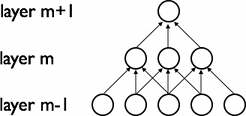
假设层m-1是输入视网膜。在上图中，层m中的单元在输入视网膜中具有宽度为3的感知野，因此仅连接到视网膜层中的3个相邻神经元。层m+1中的单元与下面的层具有类似的连接性。它们对下面的层的感知野也是3，但是它们对输入的感知野更大（5）。每个单元对视网膜感知野外的变化不响应。因此，该架构确保学习的“filter”对局部空间输入图像产生最强的响应。

然而，如上所示，堆叠许多这样的层导致（非线性）“filter”变得越来越“全局”（即响应更大的像素空间区域）。例如，隐藏层m+1中的单元可以编码宽度为5（以像素空间而言）的非线性特征。

共享权重¶

此外，在CNN中，每个filter $h_i$ 在整个视野中复制。这些复制单元共享相同的参数化（权重向量和偏差）并形成特征映射。

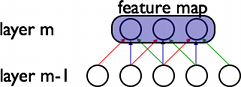
在上图中，我们显示属于同一特征映射的3个隐藏单位。相同颜色的权重相同，并且共享。梯度下降仍然可以用于学习这样的共享参数，只对原始算法有小的改变。共享权重的梯度就是被共享的参数的梯度的简单地总和。

以这种方式复制单元，使得不管特征在视野中的位置，也可以被检测到。此外，权重共享通过大大减少学习的自由参数的数量来提高学习效率。对模型的约束使CNN能够更好地泛化视觉问题。

细节和记号¶

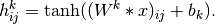
特征映射通过在整个图像的子区域上重复应用函数获得，换句话说，就是使用线性filter对输入图像进行卷积、添加偏差项、然后应用非线性函数。如果我们将给定层处的第k个特征映射表示为 $h^k$ ，其filter由权重 $W^k$ 和偏置 $b_k$ 确定，则获得的特征映射 $h^k$ 如下（对于非线性的 $tanh$ ）：

$h^k_{ij} = \tanh ( (W^k * x)_{ij} + b_k ).$

注意

回想一下1D信号的卷积的以下定义。 $o[n] = f[n]*g[n] = \sum_{u=-\infty}^{\infty} f[u] g[n-u] = \sum_{u=-\infty}^{\infty} f[n-u] g[u]$ .

这可以扩展到2D如下： $o[m,n] = f[m,n]*g[m,n] = \sum_{u=-\infty}^{\infty} \sum_{v=-\infty}^{\infty} f[u,v] g[m-u,n-v]$ 。

为了形成更丰富的数据表示，每个隐藏层由多个特征映射 $\{h^{(k)}, k=0..K\}$ 组成。隐藏层的权重 $W$ 可以用4D张量表示，该张量包含的元素对应于目的特征映射、源特征映射、源垂直位置和源水平位置的每种组合。偏置 $b$ 可以用一个向量表示，该向量包含的元素对应于每个目的地特征映射。我们用图形说明如下：

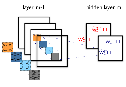
图1：卷积层的示例

该图显示了CNN的两层。层m-1包含四个特征映射。隐藏层m包含两个特征映射（ $h^0$ 和 $h^1$ ）。 $h^0$ 和 $h^1$ 中的像素（由蓝色和红色方框勾勒出）（神经元输出）从层（m-1）的像素计算出来，这些像素落入下一层的2×2接收场内（显示为彩色矩形）。注意接受场如何跨越所有四个输入特征映射。因此， $h^0$ 和 $h^1$ 的权重 $W^0$ 和 $W^1$ 是3D权重张量。主维度对输入特征映射进行索引，而其他两个维度表示像素坐标。

总之， $W^{kl}_{ij}$ 表示的权重连接m层的第k个特征映射的每个像素与层（m-1）的第l个特征映射的坐标(i, j)处的像素。

卷积运算符¶

ConvOp是在Theano中实现卷积层的主要工具。ConvOp由theano.tensor.signal.conv2d使用，它需要两个符号输入：

对应于输入图像一个mini-batch的4D张量。张量的形状如下：[mini-batch大小，输入特征映射的数量，图像高度，图像宽度]。
对应于权重矩阵 $W$ 的4D张量。张量的形状是：[层m的特征映射数，层m-1处的特征映射数，filter高度，filter宽度]

下面是用于实现类似于图1的卷积层的Theano码。输入由3个大小为120x160的特征映射（RGB颜色图像）组成。我们使用两个接受域9x9的卷积filter。

import theano
from theano import tensor as T
from theano.tensor.nnet import conv2d

import numpy

rng = numpy.random.RandomState(23455)

# instantiate 4D tensor for input
input = T.tensor4(name='input')

# initialize shared variable for weights.
w_shp = (2, 3, 9, 9)
w_bound = numpy.sqrt(3 * 9 * 9)
W = theano.shared( numpy.asarray(
            rng.uniform(
                low=-1.0 / w_bound,
                high=1.0 / w_bound,
                size=w_shp),
            dtype=input.dtype), name ='W')

# initialize shared variable for bias (1D tensor) with random values
# IMPORTANT: biases are usually initialized to zero. However in this
# particular application, we simply apply the convolutional layer to
# an image without learning the parameters. We therefore initialize
# them to random values to "simulate" learning.
b_shp = (2,)
b = theano.shared(numpy.asarray(
            rng.uniform(low=-.5, high=.5, size=b_shp),
            dtype=input.dtype), name ='b')

# build symbolic expression that computes the convolution of input with filters in w
conv_out = conv2d(input, W)

# build symbolic expression to add bias and apply activation function, i.e. produce neural net layer output
# A few words on ``dimshuffle`` :
#   ``dimshuffle`` is a powerful tool in reshaping a tensor;
#   what it allows you to do is to shuffle dimension around
#   but also to insert new ones along which the tensor will be
#   broadcastable;
#   dimshuffle('x', 2, 'x', 0, 1)
#   This will work on 3d tensors with no broadcastable
#   dimensions. The first dimension will be broadcastable,
#   then we will have the third dimension of the input tensor as
#   the second of the resulting tensor, etc. If the tensor has
#   shape (20, 30, 40), the resulting tensor will have dimensions
#   (1, 40, 1, 20, 30). (AxBxC tensor is mapped to 1xCx1xAxB tensor)
#   More examples:
#    dimshuffle('x') -> make a 0d (scalar) into a 1d vector
#    dimshuffle(0, 1) -> identity
#    dimshuffle(1, 0) -> inverts the first and second dimensions
#    dimshuffle('x', 0) -> make a row out of a 1d vector (N to 1xN)
#    dimshuffle(0, 'x') -> make a column out of a 1d vector (N to Nx1)
#    dimshuffle(2, 0, 1) -> AxBxC to CxAxB
#    dimshuffle(0, 'x', 1) -> AxB to Ax1xB
#    dimshuffle(1, 'x', 0) -> AxB to Bx1xA
output = T.nnet.sigmoid(conv_out + b.dimshuffle('x', 0, 'x', 'x'))

# create theano function to compute filtered images
f = theano.function([input], output)

让我们用这个找点乐子...

import numpy
import pylab
from PIL import Image

# open random image of dimensions 639x516
img = Image.open(open('doc/images/3wolfmoon.jpg'))
# dimensions are (height, width, channel)
img = numpy.asarray(img, dtype='float64') / 256.

# put image in 4D tensor of shape (1, 3, height, width)
img_ = img.transpose(2, 0, 1).reshape(1, 3, 639, 516)
filtered_img = f(img_)

# plot original image and first and second components of output
pylab.subplot(1, 3, 1); pylab.axis('off'); pylab.imshow(img)
pylab.gray();
# recall that the convOp output (filtered image) is actually a "minibatch",
# of size 1 here, so we take index 0 in the first dimension:
pylab.subplot(1, 3, 2); pylab.axis('off'); pylab.imshow(filtered_img[0, 0, :, :])
pylab.subplot(1, 3, 3); pylab.axis('off'); pylab.imshow(filtered_img[0, 1, :, :])
pylab.show()

这应该生成以下输出。

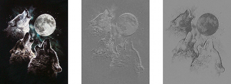
请注意，随机初始化的filter非常像边缘检测器！

注意，我们使用与MLP相同的权重初始化公式。从范围[-1/fan-in, 1 fan-in]中的均匀分布随机抽取权重，其中fan-in是隐藏单元的输入数量。对于MLP，这是下面图层中的单元数。然而，对于CNN，我们必须考虑输入特征映射的数量和接受域的大小。

MaxPooling¶

CNN的另一个重要概念是max-pooling，其是非线性向下采样的一种形式。Max-pooling将输入图像分割成一组非重叠矩形，并且对于每个这样的子区域，输出最大值。

Max-pooling在视觉中是有用的，有两个原因：

通过消除非最大值，它减少了上层的计算。
它提供了一种形式的平移不变性。想象一下，max-pooling层与卷积层级联。图像中一个像素，可以有8个方向来转换。如果max-pooling在2×2区域上完成，则这8个可能配置中的3个将在卷积层产生完全相同的输出。对于窗口为3x3的max-pooling，这变为5/8。

由于它提供了对位置的额外的鲁棒性，max-pooling是减少中间表示的维度的“聪明的”方式。

在Theano中，Max-pooling通过theano.tensor.signal.pool.pool_2d的方式完成。该函数将N维张量（其中N >= 2）和缩减因子作为输入，并且在张量最后2个维度上执行max-pooling。

一个例子值一千字：

from theano.tensor.signal import pool

input = T.dtensor4('input')
maxpool_shape = (2, 2)
pool_out = pool.pool_2d(input, maxpool_shape, ignore_border=True)
f = theano.function([input],pool_out)

invals = numpy.random.RandomState(1).rand(3, 2, 5, 5)
print 'With ignore_border set to True:'
print 'invals[0, 0, :, :] =\n', invals[0, 0, :, :]
print 'output[0, 0, :, :] =\n', f(invals)[0, 0, :, :]

pool_out = pool.pool_2d(input, maxpool_shape, ignore_border=False)
f = theano.function([input],pool_out)
print 'With ignore_border set to False:'
print 'invals[1, 0, :, :] =\n ', invals[1, 0, :, :]
print 'output[1, 0, :, :] =\n ', f(invals)[1, 0, :, :]

这应该生成以下输出：

With ignore_border set to True:
    invals[0, 0, :, :] =
    [[  4.17022005e-01   7.20324493e-01   1.14374817e-04   3.02332573e-01 1.46755891e-01]
     [  9.23385948e-02   1.86260211e-01   3.45560727e-01   3.96767474e-01 5.38816734e-01]
     [  4.19194514e-01   6.85219500e-01   2.04452250e-01   8.78117436e-01 2.73875932e-02]
     [  6.70467510e-01   4.17304802e-01   5.58689828e-01   1.40386939e-01 1.98101489e-01]
     [  8.00744569e-01   9.68261576e-01   3.13424178e-01   6.92322616e-01 8.76389152e-01]]
    output[0, 0, :, :] =
    [[ 0.72032449  0.39676747]
     [ 0.6852195   0.87811744]]

With ignore_border set to False:
    invals[1, 0, :, :] =
    [[ 0.01936696  0.67883553  0.21162812  0.26554666  0.49157316]
     [ 0.05336255  0.57411761  0.14672857  0.58930554  0.69975836]
     [ 0.10233443  0.41405599  0.69440016  0.41417927  0.04995346]
     [ 0.53589641  0.66379465  0.51488911  0.94459476  0.58655504]
     [ 0.90340192  0.1374747   0.13927635  0.80739129  0.39767684]]
    output[1, 0, :, :] =
    [[ 0.67883553  0.58930554  0.69975836]
     [ 0.66379465  0.94459476  0.58655504]
     [ 0.90340192  0.80739129  0.39767684]]

注意，与大多数Theano代码相比，max_pool_2d操作有点特殊。它需要在图构建时间知道缩减因子ds（长度2的元组，包含图像宽度和高度的缩减因子）。这可能在不久的将来改变。

完整模型：LeNet ¶

稀疏，卷积层和max-pooling是LeNet系列模型的核心。虽然模型的确切细节会有很大差异，下图显示了LeNet模型的图形描述。

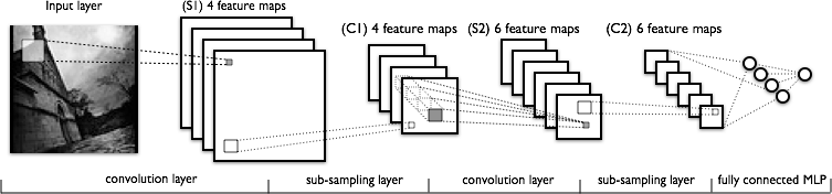
下面的层由卷积和max-pooling层交替构成。然而，上面的层是完全连接的，对应于传统的MLP（隐藏层+逻辑回归）。输入到第一个完全连接的层是下面的层的所有特征映射的集合。

从实现的角度来看，这意味着较低层对4D张量进行操作。然后将它们变平为光栅化特征图的2D矩阵，以与先前的MLP实现兼容。

注意

注意，术语“卷积”可以对应于不同的数学运算：

theano.tensor.nnet.conv2d，这是几乎所有最近发布的卷积模型中最常见的一种。在该操作中，每个输出特征映射通过不同的2D filter连接到每个输入特征映射，其值是通过相应filter对所有输入单独卷积的和。
在原始LeNet模型中使用的卷积：在此工作中，每个输出映射图仅连接到输入映射图的子集。
信号处理中使用的卷积：theano.tensor.signal.conv.conv2d，它仅适用于单通道输入。

这里，我们使用第一个操作，所以这个模型与原来的LeNet 文章略有不同。使用2.的一个原因是减少所需的计算量，但是现代硬件使得具有完全连接模式的速度一样快。另一个原因是稍微减少自由参数的数量，但我们有其它正则化技术。

合在一起¶

现在我们需要在Theano实现LeNet模型。我们从LeNetConvPoolLayer类开始，实现一个{convolution + max-pooling}层。

class LeNetConvPoolLayer(object):
    """Pool Layer of a convolutional network """

    def __init__(self, rng, input, filter_shape, image_shape, poolsize=(2, 2)):
        """
        Allocate a LeNetConvPoolLayer with shared variable internal parameters.

        :type rng: numpy.random.RandomState
        :param rng: a random number generator used to initialize weights

        :type input: theano.tensor.dtensor4
        :param input: symbolic image tensor, of shape image_shape

        :type filter_shape: tuple or list of length 4
        :param filter_shape: (number of filters, num input feature maps,
                              filter height, filter width)

        :type image_shape: tuple or list of length 4
        :param image_shape: (batch size, num input feature maps,
                             image height, image width)

        :type poolsize: tuple or list of length 2
        :param poolsize: the downsampling (pooling) factor (#rows, #cols)
        """

        assert image_shape[1] == filter_shape[1]
        self.input = input

        # there are "num input feature maps * filter height * filter width"
        # inputs to each hidden unit
        fan_in = numpy.prod(filter_shape[1:])
        # each unit in the lower layer receives a gradient from:
        # "num output feature maps * filter height * filter width" /
        #   pooling size
        fan_out = (filter_shape[0] * numpy.prod(filter_shape[2:]) //
                   numpy.prod(poolsize))
        # initialize weights with random weights
        W_bound = numpy.sqrt(6. / (fan_in + fan_out))
        self.W = theano.shared(
            numpy.asarray(
                rng.uniform(low=-W_bound, high=W_bound, size=filter_shape),
                dtype=theano.config.floatX
            ),
            borrow=True
        )

        # the bias is a 1D tensor -- one bias per output feature map
        b_values = numpy.zeros((filter_shape[0],), dtype=theano.config.floatX)
        self.b = theano.shared(value=b_values, borrow=True)

        # convolve input feature maps with filters
        conv_out = conv2d(
            input=input,
            filters=self.W,
            filter_shape=filter_shape,
            input_shape=image_shape
        )

        # pool each feature map individually, using maxpooling
        pooled_out = pool.pool_2d(
            input=conv_out,
            ds=poolsize,
            ignore_border=True
        )

        # add the bias term. Since the bias is a vector (1D array), we first
        # reshape it to a tensor of shape (1, n_filters, 1, 1). Each bias will
        # thus be broadcasted across mini-batches and feature map
        # width & height
        self.output = T.tanh(pooled_out + self.b.dimshuffle('x', 0, 'x', 'x'))

        # store parameters of this layer
        self.params = [self.W, self.b]

        # keep track of model input
        self.input = input

注意，当初始化权重值时，fan-in由接收域的大小和输入特征映射的数量确定。

最后，使用在使用逻辑回归分类MNIST数字中定义的LogisticRegression类和在多层感知器中定义的HiddenLayer类，我们可以如下实例化网络。

    x = T.matrix('x')   # the data is presented as rasterized images
    y = T.ivector('y')  # the labels are presented as 1D vector of
                        # [int] labels

    ######################
    # BUILD ACTUAL MODEL #
    ######################
    print('... building the model')

    # Reshape matrix of rasterized images of shape (batch_size, 28 * 28)
    # to a 4D tensor, compatible with our LeNetConvPoolLayer
    # (28, 28) is the size of MNIST images.
    layer0_input = x.reshape((batch_size, 1, 28, 28))

    # Construct the first convolutional pooling layer:
    # filtering reduces the image size to (28-5+1 , 28-5+1) = (24, 24)
    # maxpooling reduces this further to (24/2, 24/2) = (12, 12)
    # 4D output tensor is thus of shape (batch_size, nkerns[0], 12, 12)
    layer0 = LeNetConvPoolLayer(
        rng,
        input=layer0_input,
        image_shape=(batch_size, 1, 28, 28),
        filter_shape=(nkerns[0], 1, 5, 5),
        poolsize=(2, 2)
    )

    # Construct the second convolutional pooling layer
    # filtering reduces the image size to (12-5+1, 12-5+1) = (8, 8)
    # maxpooling reduces this further to (8/2, 8/2) = (4, 4)
    # 4D output tensor is thus of shape (batch_size, nkerns[1], 4, 4)
    layer1 = LeNetConvPoolLayer(
        rng,
        input=layer0.output,
        image_shape=(batch_size, nkerns[0], 12, 12),
        filter_shape=(nkerns[1], nkerns[0], 5, 5),
        poolsize=(2, 2)
    )

    # the HiddenLayer being fully-connected, it operates on 2D matrices of
    # shape (batch_size, num_pixels) (i.e matrix of rasterized images).
    # This will generate a matrix of shape (batch_size, nkerns[1] * 4 * 4),
    # or (500, 50 * 4 * 4) = (500, 800) with the default values.
    layer2_input = layer1.output.flatten(2)

    # construct a fully-connected sigmoidal layer
    layer2 = HiddenLayer(
        rng,
        input=layer2_input,
        n_in=nkerns[1] * 4 * 4,
        n_out=500,
        activation=T.tanh
    )

    # classify the values of the fully-connected sigmoidal layer
    layer3 = LogisticRegression(input=layer2.output, n_in=500, n_out=10)

    # the cost we minimize during training is the NLL of the model
    cost = layer3.negative_log_likelihood(y)

    # create a function to compute the mistakes that are made by the model
    test_model = theano.function(
        [index],
        layer3.errors(y),
        givens={
            x: test_set_x[index * batch_size: (index + 1) * batch_size],
            y: test_set_y[index * batch_size: (index + 1) * batch_size]
        }
    )

    validate_model = theano.function(
        [index],
        layer3.errors(y),
        givens={
            x: valid_set_x[index * batch_size: (index + 1) * batch_size],
            y: valid_set_y[index * batch_size: (index + 1) * batch_size]
        }
    )

    # create a list of all model parameters to be fit by gradient descent
    params = layer3.params + layer2.params + layer1.params + layer0.params

    # create a list of gradients for all model parameters
    grads = T.grad(cost, params)

    # train_model is a function that updates the model parameters by
    # SGD Since this model has many parameters, it would be tedious to
    # manually create an update rule for each model parameter. We thus
    # create the updates list by automatically looping over all
    # (params[i], grads[i]) pairs.
    updates = [
        (param_i, param_i - learning_rate * grad_i)
        for param_i, grad_i in zip(params, grads)
    ]

    train_model = theano.function(
        [index],
        cost,
        updates=updates,
        givens={
            x: train_set_x[index * batch_size: (index + 1) * batch_size],
            y: train_set_y[index * batch_size: (index + 1) * batch_size]
        }
    )

我们省去执行实际训练和提前停止的代码，因为它与MLP完全相同。感兴趣的读者仍然可以访问DeepLearningTutorials的'code'文件夹中的代码。

运行代码¶

然后用户可以通过以下调用来运行代码：

python code/convolutional_mlp.py

在时钟频率为3.40GHz的Core i7-2600K CPU上，使用标志“floatX=float32”，在默认参数下获得以下输出：

Optimization complete.
Best validation score of 0.910000 % obtained at iteration 17800,with test
performance 0.920000 %
The code for file convolutional_mlp.py ran for 380.28m

使用GeForce GTX 285，我们获得以下结果：

Optimization complete.
Best validation score of 0.910000 % obtained at iteration 15500,with test
performance 0.930000 %
The code for file convolutional_mlp.py ran for 46.76m

同样，在GeForce GTX 480上：

Optimization complete.
Best validation score of 0.910000 % obtained at iteration 16400,with test
performance 0.930000 %
The code for file convolutional_mlp.py ran for 32.52m

注意，验证和测试错误（以及迭代计数）的差异是由于硬件中舍入机制的不同实现。它们可以安全地忽略。

提示和技巧¶

选择超参数¶

CNNs训练特别棘手，因为它们比标准MLP增加了更多的超参数。尽管通常的学习速率和正则化常数的常用规则仍然适用，但在优化CNN时应该记住以下内容。

filter数量¶

当选择每层filter的数量时，请记住，计算单个卷积filter的激活要比传统的MLP代价高得多！

假设层 $(l-1)$ 包含 $K^{l-1}$ 个特征映射和 $M \times N$ 个像素位置（即，位置数乘以特征映射的数目），并且在 $l$ 层有 $K^l$ 个形状为形状 $m \times n$ 的filter。那么，特征映射的计算花费 $(M-m) \times (N-n) \times m \times n \times K^{l-1}$ （在所有可以应用filter的 $(M-m) \times (N-n)$ 像素位置应用一个 $m \times n$ filter）。总花费是 $K^l$ 倍。事情可能更复杂，如果一个层不是所有特征都连接到前一个的所有特征。

对于标准MLP，成本仅为 $K^l \times K^{l-1}$ ，其中在 $l$ 层存在 $K^l$ 个不同神经元。因此，CNN中使用的filter数量通常远小于MLP中的隐藏单元的数量，并且取决于特征映射的大小（其本身是输入图像大小和filter形状的函数）。

由于特征映射大小随深度减小，所以输入层附近的层将倾向于具有较少的filter，而较高的层可具有更多的filter。事实上，为了均衡每层的计算，特征的数量和像素位置的数量的乘积通常被选择为跨层大致恒定。为了保留关于输入的信息，需要保持激活的总数（特征映射的数量乘以像素位置的数量）从一层到下一层是不减少的（当然，当我们正在做监督学习时，我们希望不会减少）。特征映射的数量直接控制容量，并且这取决于可用示例的数量和任务的复杂性。

Filter形状¶

在文献中找到的常见filter的形状差异很大，通常基于数据集。在MNIST尺寸的图像（28×28）上的最佳结果第一层通常在5×5范围内，而自然图像数据集（通常在每个维度上具有数百个像素）第一层倾向于较大的filter，形状为12×12或15×15。

因此，诀窍是找到适当水平的“粒度”（即filter形状），以便在给定特定数据集的情况下以适当的比例创建抽象。

Max Pooling 形状¶

典型值为2x2或无max-pooling。非常大的输入图像在较低层中使用4x4池可能有保证。但请记住，这将会使信号的尺寸减小16倍，并且可能导致丢弃太多的信息。

脚注

[1]	为了清楚起见，我们使用词“单元”或“神经元”指人工神经元，“细胞”指生物神经元。

提示¶

如果你想在一个新的数据集上尝试这个模型，这里有一些提示，可以帮助你得到更好的结果：

白化数据（例如使用PCA）

衰减每个epoch的学习率

目录

上一主题

下一主题

这一页